Here - Stuff

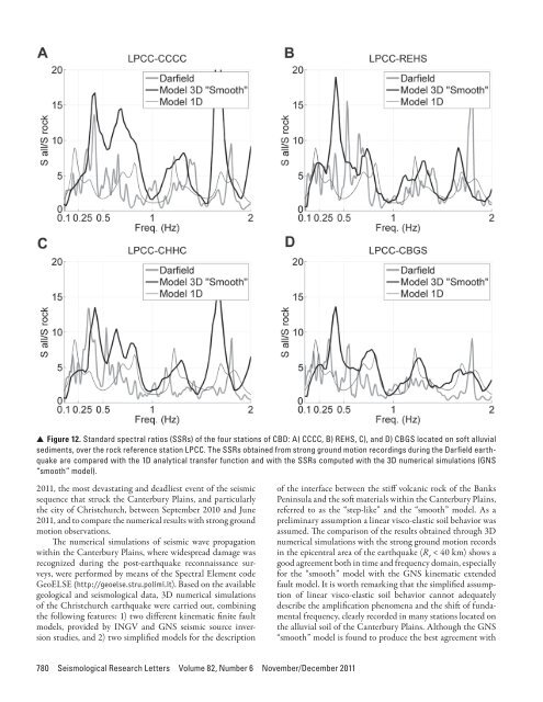
▲ ▲ Figure 12. Standard spectral ratios (SSRs) of the four stations of CBD: A) CCCC, B) REHS, C), and D) CBGS located on soft alluvialsediments, over the rock reference station LPCC. The SSRs obtained from strong ground motion recordings during the Darfield earthquakeare compared with the 1D analytical transfer function and with the SSRs computed with the 3D numerical simulations (GNS“smooth” model).2011, the most devastating and deadliest event of the seismicsequence that struck the Canterbury Plains, and particularlythe city of Christchurch, between September 2010 and June2011, and to compare the numerical results with strong groundmotion observations.The numerical simulations of seismic wave propagationwithin the Canterbury Plains, where widespread damage wasrecognized during the post-earthquake reconnaissance surveys,were performed by means of the Spectral Element codeGeoELSE (http://geoelse.stru.polimi.it). Based on the availablegeological and seismological data, 3D numerical simulationsof the Christchurch earthquake were carried out, combiningthe following features: 1) two different kinematic finite faultmodels, provided by INGV and GNS seismic source inversionstudies, and 2) two simplified models for the descriptionof the interface between the stiff volcanic rock of the BanksPeninsula and the soft materials within the Canterbury Plains,referred to as the “step-like” and the “smooth” model. As apreliminary assumption a linear visco-elastic soil behavior wasassumed. The comparison of the results obtained through 3Dnumerical simulations with the strong ground motion recordsin the epicentral area of the earthquake (R e < 40 km) shows agood agreement both in time and frequency domain, especiallyfor the “smooth” model with the GNS kinematic extendedfault model. It is worth remarking that the simplified assumptionof linear visco-elastic soil behavior cannot adequatelydescribe the amplification phenomena and the shift of fundamentalfrequency, clearly recorded in many stations located onthe alluvial soil of the Canterbury Plains. Although the GNS“smooth” model is found to produce the best agreement with780 Seismological Research Letters Volume 82, Number 6 November/December 2011