Here - Stuff
Here - Stuff Here - Stuff
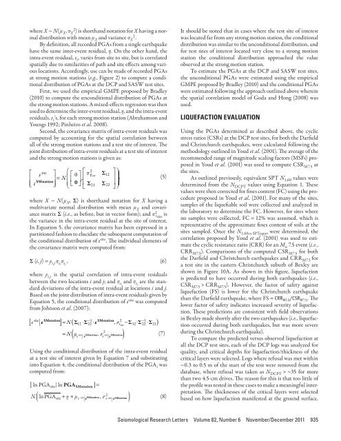
▲▲Figure 8. Aerial image of Christchurch and its environs. Superimposed on the image are locations where SASW tests were performedafter either the Darfield or the Christchurch earthquake.loading correlates to the PGA at the ground surface and theduration correlates to earthquake magnitude. Accordingly,the PGAs at the sites where DCP and SASW tests were performedneeded to be estimated for both the Darfield andthe Christchurch earthquakes. As outlined below, the PGAsrecorded at the strong motion stations (refer to Figure 2) wereused to compute the conditional PGA distribution at the testsites.The PGA at a strong motion station i can be expressed as:ln PGA i = ln PGA i (Site, Rup) + η + ε i , (3)▲ ▲ Figure 9. Measured (V S ) and corrected (V S1 ) shear wavevelocity profiles for a test site in the eastern Christchurch neighborhoodof Bexley. Also shown is the theoretical limiting upperboundvalue of V S1 for liquefaction triggering (V* S1 ) for soil havingFC = 9%.where ln(PGA i ) is the natural logarithm of the observed PGAat station i; ln PGA i (Site, Rup) is the predicted median naturallogarithm of PGA at the same station by an empirical groundmotion prediction equation (GMPE), which is a function ofthe site and earthquake rupture; η is the inter-event residual;and ε i is the intra-event residual. Based on Equation 3, empiricalGMPEs provide the distribution (unconditional) of PGAshaking as:( ) , (4)ln(PGA i )~ N ln PGA i , ση2 + σε2934 Seismological Research Letters Volume 82, Number 6 November/December 2011
where X ~ N(μ X , σ X 2 ) is shorthand notation for X having a normaldistribution with mean μ X and variance σ X 2 .By definition, all recorded PGAs from a single earthquakehave the same inter-event residual, η. On the other hand, theintra-event residual, ε i , varies from site to site, but is correlatedspatially due to similarities of path and site effects among variouslocations. Accordingly, use can be made of recorded PGAsat strong motion stations (e.g., Figure 2) to compute a conditionaldistribution of PGAs at the DCP and SASW test sites.First, we used the empirical GMPE proposed by Bradley(2010) to compute the unconditional distribution of PGAs atthe strong motion stations. A mixed-effects regression was thenused to determine the inter-event residual, η, and the intra-eventresiduals, ε i ’s, for each strong motion station (Abrahamson andYoungs 1992; Pinheiro et al. 2008).Second, the covariance matrix of intra-event residuals wascomputed by accounting for the spatial correlation betweenall of the strong motion stations and a test site of interest. Thejoint distribution of intra-event residuals at a test site of interestand the strong motion stations is given as:εsiteε = N 0 σ ε Σ0 , site 12, (5)Σ 21 Σ 22SMstation2where X ~ N(μ X , Σ) is shorthand notation for X having amultivariate normal distribution with mean μ X and covariancematrix Σ (i.e., as before, but in vector form); and σ 2 ε siteisthe variance in the intra-event residual at the site of interest.In Equation 5, the covariance matrix has been expressed in apartitioned fashion to elucidate the subsequent computation ofthe conditional distribution of ε site . The individual elements ofthe covariance matrix were computed from:Σ (i, j) = ρ i,j σ εiσ εj, (6)where ρ i,j is the spatial correlation of intra-event residualsbetween the two locations i and j; and σ εiand σ εjare the standarddeviations of the intra-event residual at locations i and j.Based on the joint distribution of intra-event residuals given byEquation 5, the conditional distribution of ε site was computedfrom Johnson et al. (2007):site SMstation1 SMstation 2[ ε ε ] = N ( Σ 12 Σ 22 ε , σεΣsite 12 Σ22 1 Σ21)= N με ε , 2(site SMstation σεsite ε ) (7)SMstationUsing the conditional distribution of the intra-event residualat a test site of interest given by Equation 7 and substitutinginto Equation 4, the conditional distribution of the PGA i wascomputed from:[ ln PGA site ln PGA SMstation ]=2( )N ln PGA site + η + μ ε σsite ε SMstation , ε site ε (8)SMstationIt should be noted that in cases where the test site of interestwas located far from any strong motion station, the conditionaldistribution was similar to the unconditional distribution, andfor test sites of interest located very close to a strong motionstation the conditional distribution approached the valueobserved at the strong motion station.To estimate the PGAs at the DCP and SASW test sites,the unconditional PGAs were estimated using the empiricalGMPE proposed by Bradley (2010) and the conditional PGAswere estimated following the approach outlined above whereinthe spatial correlation model of Goda and Hong (2008) wasused.LIQUEFACTION EVALUATIONUsing the PGAs determined as described above, the cyclicstress ratios (CSRs) at the DCP test sites, for both the Darfieldand Christchurch earthquakes, were calculated following themethodology outlined in Youd et al. (2001). The average of therecommended range of magnitude scaling factors (MSFs) proposedin Youd et al. (2001) was used to compute CSR M7.5 atthe sites.As outlined previously, equivalent SPT N 1,60 values weredetermined from the N DCPT values using Equation 1. Thesevalues were then corrected for fines content (FC) using the procedureproposed in Youd et al. (2001). For many of the sites,samples of the liquefiable soil were collected and analyzed inthe laboratory to determine the FC. However, for sites whereno samples were collected, FC = 12% was assumed, which isrepresentative of the approximate fines content of soils at thesites sampled. Once the N 1,60cs-SPTequiv were determined, thecorrelation proposed by Youd et al. (2001) was used to estimatethe cyclic resistance ratio (CRR) for an M w 7.5 event (i.e.,CRR M7.5 ). Comparisons of the computed CSR M7.5 for boththe Darfield and Christchurch earthquakes and CRR M7.5 fora test site in the eastern Christchurch suburb of Bexley areshown in Figure 10A. As shown in this figure, liquefactionis predicted to have occurred during both earthquakes (i.e.,CSR M7.5 > CRR M7.5 ). However, the factor of safety againstliquefaction (FS) is lower for the Christchurch earthquakethan the Darfield earthquake, where FS = CRR M7.5 /CSR M7.5 . Thelower factor of safety indicates increased severity of liquefaction.These predictions are consistent with field observationsin Bexley made shortly after the two earthquakes (i.e., liquefactionoccurred during both earthquakes, but was more severeduring the Christchurch earthquake).To compare the predicted versus observed liquefaction atall the DCP test sites, each of the DCP logs was analyzed forquality, and critical depths for liquefaction/thickness of thecritical layers were selected. Logs where refusal was met within~0.3 to 0.5 m of the start of the test were removed from thedatabase, where refusal was taken as N DCPT > ~35 for morethan two 4.5-cm drives. The reason for this is that too little ofthe profile was tested in these cases to make a meaningful interpretation.The thicknesses of the critical layers were selectedbased on how liquefaction manifested at the ground surface.Seismological Research Letters Volume 82, Number 6 November/December 2011 935
- Page 129 and 130: (A)(B)(C)(D)(E)▲▲Figure 1. A) M
- Page 131 and 132: (A) (B) (C)▲ ▲ Figure 3. A) Typ
- Page 133 and 134: (A) (B) (C)▲ ▲ Figure 4. A) Typ
- Page 135 and 136: Case StudyKey ParametersTABLE 1Key
- Page 137 and 138: ▲ ▲ Figure 9. Representative bu
- Page 139 and 140: Soil Liquefaction Effects in the Ce
- Page 141 and 142: ▲ ▲ Figure 2. Representative su
- Page 143 and 144: Location of structures illustrated
- Page 145 and 146: Shading indicates areaover which pr
- Page 147 and 148: 1.8 deg15 cmGround cracking due to
- Page 149 and 150: 30 cm17 cm30 cmFoundation beam▲
- Page 151 and 152: Comparison of Liquefaction Features
- Page 153 and 154: (A)(B)▲▲Figure 2. A) Simplified
- Page 155 and 156: (A)Acceleration (Gal)6004002000-200
- Page 157 and 158: (A)(B)▲▲Figure 7. Distribution
- Page 159 and 160: (A)(B)▲▲Figure 10. Damage to a
- Page 161 and 162: (A)(B)▲ ▲ Figure 14. A) Subside
- Page 163 and 164: ▲▲Figure 17. A trench in a resi
- Page 165 and 166: Ambient Noise Measurements followin
- Page 167 and 168: ▲▲Figure 1. Location of the noi
- Page 169 and 170: ▲▲Figure 5. Site N20 showing HV
- Page 171 and 172: ▲▲Figure 8. Comparison between
- Page 173 and 174: Use of DCP and SASW Tests to Evalua
- Page 175 and 176: ▲ ▲ Figure 2. Aerial image of C
- Page 177 and 178: (A)(B)▲▲Figure 4. DCP test bein
- Page 179: ▲▲Figure 7. SASW setup at a sit
- Page 183 and 184: Using the same critical layers as s
- Page 185 and 186: Performance of Levees (Stopbanks) d
- Page 187 and 188: ▲▲Figure 3. Typical geometry an
- Page 189 and 190: TABLE 1Damage severity categories (
- Page 191 and 192: (A)(B)▲▲Figure 6. A) Large sand
- Page 193 and 194: (A)(B)▲▲Figure 8. A) Representa
- Page 195 and 196: each of the Waimakariri River and a
- Page 197 and 198: ▲ ▲ Figure 2. Horizontal peak g
- Page 199 and 200: only minor damage, mostly to their
- Page 201 and 202: (A)(C)(B)▲▲Figure 5. Ferrymead
- Page 203 and 204: (A)(B)▲▲Figure 7. Damage to sou
- Page 205 and 206: (A)(B)▲▲Figure 11. Settlement o
- Page 207 and 208: (A)(C)(B)▲▲Figure 14. Railway B
- Page 209 and 210: Events Reconnaissance (GEER) Associ
- Page 211 and 212: New PublicationsCanGeoRefThe Americ
- Page 213 and 214: Wednesday, 18 AprilTechnical Sessio
- Page 215 and 216: Verification of a Spectral-Element
- Page 217 and 218: EASTERN SECTIONRESEARCH LETTERSReas
- Page 219 and 220: (A)70°N100°W 60°W70°N(B)100°E1
- Page 221 and 222: Mongolia SCRThe presence or absence
- Page 223 and 224: the small horizontal relative motio
- Page 225 and 226: 80°100°120°140°EXPLANATIONBorde
- Page 227 and 228: Chang, K. H. (1997). Korean peninsu
- Page 229 and 230: Wheeler, R. L. (2008). Paleoseismic
where X ~ N(μ X , σ X 2 ) is shorthand notation for X having a normaldistribution with mean μ X and variance σ X 2 .By definition, all recorded PGAs from a single earthquakehave the same inter-event residual, η. On the other hand, theintra-event residual, ε i , varies from site to site, but is correlatedspatially due to similarities of path and site effects among variouslocations. Accordingly, use can be made of recorded PGAsat strong motion stations (e.g., Figure 2) to compute a conditionaldistribution of PGAs at the DCP and SASW test sites.First, we used the empirical GMPE proposed by Bradley(2010) to compute the unconditional distribution of PGAs atthe strong motion stations. A mixed-effects regression was thenused to determine the inter-event residual, η, and the intra-eventresiduals, ε i ’s, for each strong motion station (Abrahamson andYoungs 1992; Pinheiro et al. 2008).Second, the covariance matrix of intra-event residuals wascomputed by accounting for the spatial correlation betweenall of the strong motion stations and a test site of interest. Thejoint distribution of intra-event residuals at a test site of interestand the strong motion stations is given as:εsiteε = N 0 σ ε Σ0 , site 12, (5)Σ 21 Σ 22SMstation2where X ~ N(μ X , Σ) is shorthand notation for X having amultivariate normal distribution with mean μ X and covariancematrix Σ (i.e., as before, but in vector form); and σ 2 ε siteisthe variance in the intra-event residual at the site of interest.In Equation 5, the covariance matrix has been expressed in apartitioned fashion to elucidate the subsequent computation ofthe conditional distribution of ε site . The individual elements ofthe covariance matrix were computed from:Σ (i, j) = ρ i,j σ εiσ εj, (6)where ρ i,j is the spatial correlation of intra-event residualsbetween the two locations i and j; and σ εiand σ εjare the standarddeviations of the intra-event residual at locations i and j.Based on the joint distribution of intra-event residuals given byEquation 5, the conditional distribution of ε site was computedfrom Johnson et al. (2007):site SMstation1 SMstation 2[ ε ε ] = N ( Σ 12 Σ 22 ε , σεΣsite 12 Σ22 1 Σ21)= N με ε , 2(site SMstation σεsite ε ) (7)SMstationUsing the conditional distribution of the intra-event residualat a test site of interest given by Equation 7 and substitutinginto Equation 4, the conditional distribution of the PGA i wascomputed from:[ ln PGA site ln PGA SMstation ]=2( )N ln PGA site + η + μ ε σsite ε SMstation , ε site ε (8)SMstationIt should be noted that in cases where the test site of interestwas located far from any strong motion station, the conditionaldistribution was similar to the unconditional distribution, andfor test sites of interest located very close to a strong motionstation the conditional distribution approached the valueobserved at the strong motion station.To estimate the PGAs at the DCP and SASW test sites,the unconditional PGAs were estimated using the empiricalGMPE proposed by Bradley (2010) and the conditional PGAswere estimated following the approach outlined above whereinthe spatial correlation model of Goda and Hong (2008) wasused.LIQUEFACTION EVALUATIONUsing the PGAs determined as described above, the cyclicstress ratios (CSRs) at the DCP test sites, for both the Darfieldand Christchurch earthquakes, were calculated following themethodology outlined in Youd et al. (2001). The average of therecommended range of magnitude scaling factors (MSFs) proposedin Youd et al. (2001) was used to compute CSR M7.5 atthe sites.As outlined previously, equivalent SPT N 1,60 values weredetermined from the N DCPT values using Equation 1. Thesevalues were then corrected for fines content (FC) using the procedureproposed in Youd et al. (2001). For many of the sites,samples of the liquefiable soil were collected and analyzed inthe laboratory to determine the FC. However, for sites whereno samples were collected, FC = 12% was assumed, which isrepresentative of the approximate fines content of soils at thesites sampled. Once the N 1,60cs-SPTequiv were determined, thecorrelation proposed by Youd et al. (2001) was used to estimatethe cyclic resistance ratio (CRR) for an M w 7.5 event (i.e.,CRR M7.5 ). Comparisons of the computed CSR M7.5 for boththe Darfield and Christchurch earthquakes and CRR M7.5 fora test site in the eastern Christchurch suburb of Bexley areshown in Figure 10A. As shown in this figure, liquefactionis predicted to have occurred during both earthquakes (i.e.,CSR M7.5 > CRR M7.5 ). However, the factor of safety againstliquefaction (FS) is lower for the Christchurch earthquakethan the Darfield earthquake, where FS = CRR M7.5 /CSR M7.5 . Thelower factor of safety indicates increased severity of liquefaction.These predictions are consistent with field observationsin Bexley made shortly after the two earthquakes (i.e., liquefactionoccurred during both earthquakes, but was more severeduring the Christchurch earthquake).To compare the predicted versus observed liquefaction atall the DCP test sites, each of the DCP logs was analyzed forquality, and critical depths for liquefaction/thickness of thecritical layers were selected. Logs where refusal was met within~0.3 to 0.5 m of the start of the test were removed from thedatabase, where refusal was taken as N DCPT > ~35 for morethan two 4.5-cm drives. The reason for this is that too little ofthe profile was tested in these cases to make a meaningful interpretation.The thicknesses of the critical layers were selectedbased on how liquefaction manifested at the ground surface.Seismological Research Letters Volume 82, Number 6 November/December 2011 935


