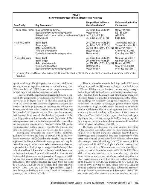
(A)(D)(B)(C)▲ ▲ Figure 5. A) The CBGS seismic station, with the remnants of liquefaction sand boils seen as scars on the grass. B) Accelerationtime histories of CBGS: record and analysis. C) Comparison of the above acceleration time histories after filtering them at 4 Hz. D)Comparison of 5% damped spectra between CBGS record and analysis.the building stock in the CBD, representing short-, medium-,and long-period structures. Our goal is not, obviously, to studyin detail certain structures but to “reconcile” earthquake damagewith ground motions. One- and two-story timber residentialhouses and two RC frame structures of different height,one six stories and one 17 stories, have been examined “generically”as described below in detail. Another case study couldselect URM buildings, a fairly representative typology in CBD,which suffered much from out-of-plane wall failures.The selected buildings are treated as reference structuresfor their category, while the variability in the structural characteristicswithin each structural category is assumed to follow astatistical distribution simulated through a Monte-Carlo algorithm.This approach is a necessity since at this stage detailedstructural data are not available. The parameters of the statisticaldistribution, i.e., mean value, coefficient of variation, typeof distribution, etc., are either taken from the available literatureor estimated using engineering judgment guided by the(macroscopic) visual inspection. The assumed values, as well asthe relative references for each parameter and structural categoryexamined, are summarized in Table 1.Having created a large number of simulated buildings, weapplied the displacement-based assessment procedure establishedby Priestley et al. (2007) to evaluate the demand on eachbuilding. This is then translated to displacement demands foreach floor and to inter-story drifts, utilizing the displacementprofiles proposed in Priestley et al. (2007). The method is basedon the substitute-structure theory, first suggested by Gülkan andSözen (1974) and Shibata and Sözen (1976), according to whichan inelastic multi-degree-of-freedom (MDOF) system can berepresented by an equivalent inelastic single-degree-of-freedomsystem (SDOF). The only aspect of our methodology that, outof necessity, deviates from the Priestley et al. (2007) is that the“yield period” of each structural category is based on literaturesuggestions rather than an initial estimate of stiffness and themass of each specific building. The “yield period” refers to thestiffness at the point of yielding, which is the limit beyond whichsubstantial inelastic response begins that eventually may lead to888 Seismological Research Letters Volume 82, Number 6 November/December 2011
Case StudyKey ParametersTABLE 1Key Parameters Used in the Representative Analyses1- and 2-story timber Displacement limit statesEquivalent viscous damping equationRatio of the first yield to the base shear coefficientStory height6-story RC frame17-story RC frameBeam depthBeam lengthRebar yield strengthYield-period equationEquivalent viscous damping equationBeam depthBeam lengthRebar yield strengthYield-period equationEquivalent viscous damping equationRanges Used in MonteCarlo Simulations *µ = 8 mm, CoV = 0.15, [N]Deterministica = 0.5, b = 0.8, [U]a = 2.8 m, b = 3.1 m, [U]µ = 0.8 m, CoV = 0.15, [N]µ = 7.0 m, CoV = 0.15, [N]µ = 330 MPa, CoV = 0.15, [N]DeterministicDeterministicµ = 0.6 m, CoV = 0.15, [N]µ = 5.0 m, CoV = 0.15, [N]µ = 330 MPa, CoV = 0.15, [N]DeterministicDeterministicReference for the KeyParametersUma et al. 2008NZSEE 2006ATC 1996Field dataTasiopoulou et al. 2011Tasiopoulou et al. 2011Uma et al. 2008Crowley et al. 2004Priestley et al. 2007Galloway et al. 2011Galloway et al. 2011Uma et al. 2008Crowley et al. 2004Priestley et al. 2007* µ: mean, CoV: coefficient of variation, [N]: Normal distribution, [U]: Uniform distribution, a and b: limits of the uniform distribution.significant damage. The yield period has been successfully usedas a key parameter in performance assessment by Crowley et al.(2004) and Bal et al. (2010). References for the parameters usedfor each category of buildings are given in Table 1.To ensure that the maximum displacement demand is estimated,the components for each record have been rotated inincrements of 1° degree from 0° to 180°, thus creating a newset of 180 records and the corresponding response spectra. Thecontours of the maps presented in the paper (see Figures 6 to8) have been derived after assessing each simulated buildingfor a total of 180 response spectra. Note that the inter-storydrift demands have been calculated only at the position of therecording stations, as shown on the maps in Figures 6 to 8. Thevalues presented between the stations are only the result of linearinterpolation among several “anchor” points. Obviously,the interpolation in these figures is bound by the coastline andcannot be extended to Kaiapoi and to Lyttelton Port stations.Short-period structures are mostly timber buildings.Such two-story houses are found in the CBD, while one-storyhouses are outside the CBD and in the suburbs. They are nonengineeredbuildings, with few if any exceptions; local regulationsallow simple timber houses to be constructed without anapproved design. Both groups were significantly damaged, butonly a few collapsed. However, the damage to such houses dueto liquefaction-induced ground differential settlements andhorizontal displacements was unprecedented. A generic buildinghas been used in this study as a reference structure. Theproperties of this generic structure are taken from the workby Uma et al. (2008), in which the story drift limits are givenas 0.3%, 0.6%, 1.2%, and 1.6% for slight, moderate, significantdamage, and collapse limit states. Details of the assumedparameters can be found in Table 1.There are several commercial buildings in the CBD, mostof which are mid-rise RC structures designed and built in the1970s and 1980s when the developed modern design conceptshad only partially (at best) been incorporated in codes. A specificbuilding from Kilmore Street (Markham’s Building),shown in Figure 9, is used for generating an ensemble of similarbuildings for moderately long-period structures. Despitewidespread liquefaction in the area, its pile foundation helpedto limit the damage; thus, the results presented below refer tosimilar buildings founded on stable upper soil layers. The finalcase study is a real building in Worchester Street, known asClarendon Tower, which has been reported to have undergonesignificant but repairable damage in the February earthquake.It is a regular moment-resisting frame structure, the details ofwhich are given in Galloway et al. (2011).The spatial distribution of the mean values of inter-storydrift demands in Christchurch for two-story timber structures(Figure 6), computed using the approach described above,clearly suggests that there must have been concentration of theinter-story demand in and near the Heathcote Valley wherethe strongest recorded shaking (HVSC) in terms of PGAand low-period SA and SD took place. On the contrary, damagein the area of the CBD must have been somewhat lighter,apparently due to the smaller low-period SD in the CBD. Suchdifferences can be attributed to the somewhat larger distancefrom the source and the fact that the soft soils de-amplified theshort-period seismic waves. But still, the median inter-storydrift demands in the CBD are computed to have been in theorder of 1.0%–1.5% for two-story timber structures, a level ofdemand definitely sufficient to induce substantial structuraldamage. Indeed, observations from different parts of the CBDon a variety of timber two-story structures confirm this theo-Seismological Research Letters Volume 82, Number 6 November/December 2011 889
- Page 1:
Volume 82, Number 6 November/Decemb
- Page 7:
News and Notes (continued)Nominatio
- Page 11:
Preface to the Focused Issue on the
- Page 14 and 15:
TABLE 1Peak ground acceleration (PG
- Page 16 and 17:
▲▲Figure 2. A) Sketch of the
- Page 18 and 19:
▲▲Figure 4. A) Adopted moment r
- Page 20 and 21:
▲▲Figure 7. As in Figure 6 but
- Page 22 and 23:
▲ ▲ Figure 8. Misfit parameters
- Page 24 and 25:
▲ ▲ Figure 10. Spatial variabil
- Page 26 and 27:
▲ ▲ Figure 12. Standard spectra
- Page 28 and 29:
Quigley, M., R. Van Dissen, P. Vill
- Page 30 and 31:
slip on a 59-degree striking fault
- Page 32 and 33:
▲▲Figure 4. Convergence of inve
- Page 34 and 35:
observations and other source studi
- Page 36 and 37:
-42. 5-43. 0-43. 5-44. 0-44. 5-43.2
- Page 38 and 39:
“Product CSK © ASI, (ItalianSpac
- Page 40 and 41:
TABLE 2Solutions for fault location
- Page 42 and 43:
-43.45(A)degrees N-43.50-43.552.52.
- Page 44 and 45:
is still a good fit to the horizont
- Page 46 and 47:
Coulomb Stress Change Sensitivity d
- Page 48 and 49:
mation takes on a larger strike-sli
- Page 50 and 51:
P 9.4267BLDU45P 20.1213CASY39P 2.62
- Page 52 and 53:
ERMJNUMAJOINUJHJ2CBIJMIDWJOWYHNBTPU
- Page 54 and 55:
(A)6.146.13(B)6.246.36Misfit6.156.1
- Page 56 and 57:
(A)(B)(C)(D)▲▲Figure 10. The co
- Page 58 and 59:
(A)(B)(C)(D)▲▲Figure 12. The co
- Page 60 and 61:
Luo, Y., Y. Tan, S. Wei, D. Helmber
- Page 62 and 63:
−44˚00' −43˚00'4-Sep-2010Mw 7
- Page 64 and 65:
TABLE 1Pairs of SAR imagery used in
- Page 67 and 68:
Depth (km)Coulomb Stress Change(bar
- Page 69 and 70:
Crippen, R. E. (1992). Measurement
- Page 71 and 72:
AlpineFaultHope Fault38 mm/yr0+ +-1
- Page 73 and 74:
σ 1dσ 3Nuσ 3CM w 7.1dw 6.2u70°M
- Page 75 and 76:
Right-lateral Faults(A) Range Front
- Page 77 and 78:
DISCUSSIONThe 2010-2011 Canterbury
- Page 79 and 80:
Large Apparent Stresses from the Ca
- Page 81 and 82:
▲ ▲ Figure 2. Observed vs. pred
- Page 83 and 84: 10Obs SA(1s)AS1AS+SDAB 2006AB+SDSA(
- Page 85 and 86: Fine-scale Relocation of Aftershock
- Page 87 and 88: −43.25°OXZ0 10 20km−43.5°−4
- Page 89 and 90: A’0 km 4 8−43.5°B’B−43.6°
- Page 91 and 92: REFERENCESAvery, H. R., J. B. Berri
- Page 93 and 94: ▲ ▲ Figure 2. A) shows three-co
- Page 95 and 96: ▲ ▲ Figure 4. Vertical accelera
- Page 97 and 98: 0.8PRPC Z0.40Normalized (Max PGA +
- Page 99 and 100: Near-source Strong Ground MotionsOb
- Page 101 and 102: (A)Magnitude, M w876542009 NZdataba
- Page 103 and 104: Scale0.5 g5 seconds▲▲Figure 4.
- Page 105 and 106: (A)(B)Spectral Acc, Sa (g)North/Wes
- Page 107 and 108: Vertical-to-horizontal PGA ratio543
- Page 109 and 110: (A)(B)Station:CCCCSolid:AvgHorizDas
- Page 111 and 112: REFERENCESAagaard, B. T., J. F. Hal
- Page 113 and 114: ▲ ▲ Figure 1. Shear-wave veloci
- Page 115 and 116: Spectral Acceleration (0.3 s), (g)I
- Page 117 and 118: Spectral Acceleration (3 s), (g)In[
- Page 119 and 120: TABLE 1Mean (μ LLH ) and standard
- Page 121 and 122: Strong Ground Motions and Damage Co
- Page 123 and 124: ings and the Modified Takeda-Slip M
- Page 125 and 126: high, but there were no buildings d
- Page 127 and 128: REFERENCES▲▲Figure 8. Heavily d
- Page 129 and 130: (A)(B)(C)(D)(E)▲▲Figure 1. A) M
- Page 131 and 132: (A) (B) (C)▲ ▲ Figure 3. A) Typ
- Page 133: (A) (B) (C)▲ ▲ Figure 4. A) Typ
- Page 137 and 138: ▲ ▲ Figure 9. Representative bu
- Page 139 and 140: Soil Liquefaction Effects in the Ce
- Page 141 and 142: ▲ ▲ Figure 2. Representative su
- Page 143 and 144: Location of structures illustrated
- Page 145 and 146: Shading indicates areaover which pr
- Page 147 and 148: 1.8 deg15 cmGround cracking due to
- Page 149 and 150: 30 cm17 cm30 cmFoundation beam▲
- Page 151 and 152: Comparison of Liquefaction Features
- Page 153 and 154: (A)(B)▲▲Figure 2. A) Simplified
- Page 155 and 156: (A)Acceleration (Gal)6004002000-200
- Page 157 and 158: (A)(B)▲▲Figure 7. Distribution
- Page 159 and 160: (A)(B)▲▲Figure 10. Damage to a
- Page 161 and 162: (A)(B)▲ ▲ Figure 14. A) Subside
- Page 163 and 164: ▲▲Figure 17. A trench in a resi
- Page 165 and 166: Ambient Noise Measurements followin
- Page 167 and 168: ▲▲Figure 1. Location of the noi
- Page 169 and 170: ▲▲Figure 5. Site N20 showing HV
- Page 171 and 172: ▲▲Figure 8. Comparison between
- Page 173 and 174: Use of DCP and SASW Tests to Evalua
- Page 175 and 176: ▲ ▲ Figure 2. Aerial image of C
- Page 177 and 178: (A)(B)▲▲Figure 4. DCP test bein
- Page 179 and 180: ▲▲Figure 7. SASW setup at a sit
- Page 181 and 182: where X ~ N(μ X , σ X 2 ) is shor
- Page 183 and 184: Using the same critical layers as s
- Page 185 and 186:
Performance of Levees (Stopbanks) d
- Page 187 and 188:
▲▲Figure 3. Typical geometry an
- Page 189 and 190:
TABLE 1Damage severity categories (
- Page 191 and 192:
(A)(B)▲▲Figure 6. A) Large sand
- Page 193 and 194:
(A)(B)▲▲Figure 8. A) Representa
- Page 195 and 196:
each of the Waimakariri River and a
- Page 197 and 198:
▲ ▲ Figure 2. Horizontal peak g
- Page 199 and 200:
only minor damage, mostly to their
- Page 201 and 202:
(A)(C)(B)▲▲Figure 5. Ferrymead
- Page 203 and 204:
(A)(B)▲▲Figure 7. Damage to sou
- Page 205 and 206:
(A)(B)▲▲Figure 11. Settlement o
- Page 207 and 208:
(A)(C)(B)▲▲Figure 14. Railway B
- Page 209 and 210:
Events Reconnaissance (GEER) Associ
- Page 211 and 212:
New PublicationsCanGeoRefThe Americ
- Page 213 and 214:
Wednesday, 18 AprilTechnical Sessio
- Page 215 and 216:
Verification of a Spectral-Element
- Page 217 and 218:
EASTERN SECTIONRESEARCH LETTERSReas
- Page 219 and 220:
(A)70°N100°W 60°W70°N(B)100°E1
- Page 221 and 222:
Mongolia SCRThe presence or absence
- Page 223 and 224:
the small horizontal relative motio
- Page 225 and 226:
80°100°120°140°EXPLANATIONBorde
- Page 227 and 228:
Chang, K. H. (1997). Korean peninsu
- Page 229 and 230:
Wheeler, R. L. (2008). Paleoseismic
- Page 231 and 232:
A significant outcome of this study
- Page 233 and 234:
TABLE 1 (continued)Earthquakes for
- Page 235 and 236:
▲▲Figure 2. Earthquakes used in
- Page 237 and 238:
Meeting CalendarM E E T I N GC A L
- Page 239 and 240:
201 Plaza Professional Bldg. • El
- Page 241 and 242:
Seismological Research Letters (SRL
- Page 243 and 244:
Christa von Hillebrandt-Andrade, Pr