geothermal power plant projects in central america - Orkustofnun
geothermal power plant projects in central america - Orkustofnun geothermal power plant projects in central america - Orkustofnun
average results, and combining them with data from Central America (Bloomfield and Laney, 2005), itis possible to estimate the expected value and its limits of error for drilling investment in this region.Stefansson (2002) stated that the average yield of wells in any particular geothermal field is fairlyconstant after passing through a certain learning period and gaining sufficient knowledge of thereservoir to site the wells so as to achieve the maximum possible yield. The average power output(MW) per drilled kilometer in geothermal fields is shown as a function of the number of wells in eachfield.TABLE 6: Average values for 31 geothermal fields (Stefansson, 2002)Average MW per well 4.2 ± 2.2Average MW per drilled km 3.4 ± 1.4Average number of wells before max. yield achieved 9.3 ± 6.1For this estimation, it is assumed that the average depth of the wells is 1,890 m, and that the averagecost of such wells is 3.24 million USD as presented in Table 2 (drilling costs in Central America asreported by Bloomfield and Laney, 2005).TABLE 7: Drilling costs from 1997 to 2000 for Central America and the Azores in 2010 USD(Bloomfield and Laney, 2005)DepthInterval(km)NumberofWellsTotalCost(MUSD)AverageDepth(km)AverageCost/Well(MUSD)0.00–0.38 1 0.33 0.21 0.330.38–0.76 8 12.34 0.60 1.540.76–1.14 0 0.00 0.00 0.001.14–1.52 5 12.87 1.31 2.571.52–2.28 24 77.13 1.77 3.212.28–3.04 20 81.57 2.55 4.083.04–3.81 3 13.62 3.35 4.54Total1.89 3.24The average yield of the 1,890 m wells is 3.24 x (3.4±1.4) = (6.43 ±2.6) MW, and the cost per MW is3.24 / (6.43 ±2.6) = 0.5 (+0.46/-0.21) MUSD/MW.According to Stefansson (2002) this cost per MW is relatively insensitive to the drilling depth (anddrilling cost) because the yield of the wells refers to each km drilled; for the first step of fielddevelopment, the learning cost has to be added to the cost estimate. This cost is associated withdrilling a sufficient number of wells in order to know where to site the wells for a maximum yieldfrom drilling. As shown in Table 6, the average number of wells required for this is 9.3±6.1 wells.Assuming that the average yield in the learning period is 50%, 4.6±3.0 wells are adding to the firstdevelopment step. Incorporating the average cost per well, shown in Table 7, the additional cost is15.07±9.7 million USD. The estimation for expected drilling investment cost is calculated as follows: = (15.07 ± 9.7) + [(0.5 + 0.46/−0.21) ∗ ] (35)Using 2010 USD values, the cost of wells has been inflated according to the US BLS (2011) inflationcalculator.5.4 Power plantEquipment purchase cost estimation is the key driver of the capital cost estimation for a given powerplant project. There are three main sources of equipment estimation data: vendor contacts, open29
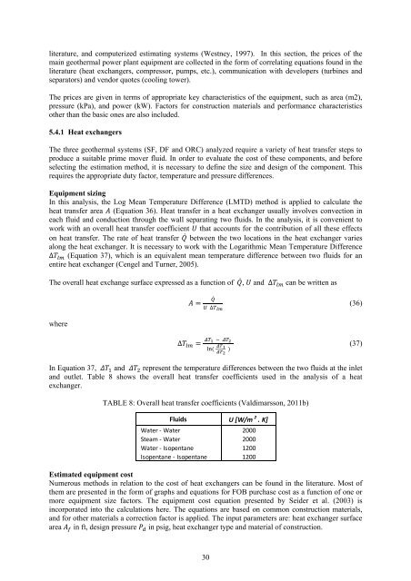
literature, and computerized estimating systems (Westney, 1997). In this section, the prices of themain geothermal power plant equipment are collected in the form of correlating equations found in theliterature (heat exchangers, compressor, pumps, etc.), communication with developers (turbines andseparators) and vendor quotes (cooling tower).The prices are given in terms of appropriate key characteristics of the equipment, such as area (m2),pressure (kPa), and power (kW). Factors for construction materials and performance characteristicsother than the basic ones are also included.5.4.1 Heat exchangersThe three geothermal systems (SF, DF and ORC) analyzed require a variety of heat transfer steps toproduce a suitable prime mover fluid. In order to evaluate the cost of these components, and beforeselecting the estimation method, it is necessary to define the size and design of the component. Thisrequires the appropriate duty factor, temperature and pressure differences.Equipment sizingIn this analysis, the Log Mean Temperature Difference (LMTD) method is applied to calculate theheat transfer area (Equation 36). Heat transfer in a heat exchanger usually involves convection ineach fluid and conduction through the wall separating two fluids. In the analysis, it is convenient towork with an overall heat transfer coefficient that accounts for the contribution of all these effectson heat transfer. The rate of heat transfer between the two locations in the heat exchanger variesalong the heat exchanger. It is necessary to work with the Logarithmic Mean Temperature Difference∆ (Equation 37), which is an equivalent mean temperature difference between two fluids for anentire heat exchanger (Cengel and Turner, 2005).The overall heat exchange surface expressed as a function of , and ∆ can be written aswhere= ∆ (36)∆ = ( ) (37)In Equation 37, and represent the temperature differences between the two fluids at the inletand outlet. Table 8 shows the overall heat transfer coefficients used in the analysis of a heatexchanger.TABLE 8: Overall heat transfer coefficients (Valdimarsson, 2011b)Fluids U [W/m 2 . K]Water - Water 2000Steam - Water 2000Water - Isopentane 1200Isopentane - Isopentane 1200Estimated equipment costNumerous methods in relation to the cost of heat exchangers can be found in the literature. Most ofthem are presented in the form of graphs and equations for FOB purchase cost as a function of one ormore equipment size factors. The equipment cost equation presented by Seider et al. (2003) isincorporated into the calculations here. The equations are based on common construction materials,and for other materials a correction factor is applied. The input parameters are: heat exchanger surfacearea in ft, design pressure in psig, heat exchanger type and material of construction.30
- Page 1 and 2: GEOTHERMAL TRAINING PROGRAMMEHot sp
- Page 3 and 4: This MSc thesis has also been publi
- Page 5 and 6: ACKNOWLEDGEMENTSMy gratitude to the
- Page 7 and 8: TABLE OF CONTENTSPage1. INTRODUCTIO
- Page 9 and 10: PageAPPENDIX A: FINANCIAL MODEL ...
- Page 12 and 13: 1. INTRODUCTIONRecent research on r
- Page 14 and 15: 2. CENTRAL AMERICAN DATA2.1 Power p
- Page 16 and 17: 2.2.3 HondurasThe Honduran electric
- Page 18 and 19: NET INJECTION BY SOURCE (2010)INSTA
- Page 20 and 21: income taxes for a period of 10 yea
- Page 22 and 23: annual temperature ranges from 17 t
- Page 24 and 25: egional reconnaissance in 1981ident
- Page 26 and 27: 4. GEOTHERMAL ELECTRICAL POWER ASSE
- Page 28 and 29: The net contribution of that power
- Page 30 and 31: Introducing , = , and , = ,
- Page 32 and 33: 9ProductionWellBoiler5Turbine~1046P
- Page 34 and 35: TABLE 3: Parameters and boundary co
- Page 36 and 37: eaches the maximum limit, and for h
- Page 38 and 39: 160180140160tc vap[i], th vap[i]120
- Page 42 and 43: The base cost ( ) can be calculate
- Page 44 and 45: calculation for another separator c
- Page 46 and 47: mass flow rate (kg/s) on the plant
- Page 48 and 49: Table 11 shows a summary of costs f
- Page 50 and 51: 5.6.4 Comparison of capital costs b
- Page 52 and 53: 6. FINANCIAL FEASIBILITY ASSESSMENT
- Page 54 and 55: 6.2 Model structureThe financial fe
- Page 56 and 57: CCF = EBITDA − ∆Working Capital
- Page 58 and 59: Interest on loansFleischmann (2007)
- Page 60 and 61: IRR30%25%IRR CapitalIRR Equity20%Si
- Page 62 and 63: FIGURE 42: Allocation of funds for:
- Page 64 and 65: 340IRR Free Cash Flow to Equity [ %
- Page 66 and 67: flash technology is between 0.3 and
- Page 68 and 69: Energy Price Availability Factor O&
- Page 70 and 71: FIGURE 50: Density and cumulative p
- Page 72 and 73: In Chapter 6, Figure 44 illustrated
- Page 74 and 75: The internal rate of return is offs
- Page 76 and 77: Cengel, Y. and Tuner, R., 2005: Fun
- Page 78 and 79: IEAb, 2011: Technology roadmap: Geo
- Page 80 and 81: Salmon, J., Meurice, J., Wobus, N.,
- Page 82 and 83: APPENDIX A: SUMMARY OF FINANCIAL MO
- Page 84 and 85: APPENDIX C: INVESTMENT AND FINANCIN
- Page 86 and 87: APPENDIX E: BALANCE SHEETBALANCE SH
literature, and computerized estimat<strong>in</strong>g systems (Westney, 1997). In this section, the prices of thema<strong>in</strong> <strong>geothermal</strong> <strong>power</strong> <strong>plant</strong> equipment are collected <strong>in</strong> the form of correlat<strong>in</strong>g equations found <strong>in</strong> theliterature (heat exchangers, compressor, pumps, etc.), communication with developers (turb<strong>in</strong>es andseparators) and vendor quotes (cool<strong>in</strong>g tower).The prices are given <strong>in</strong> terms of appropriate key characteristics of the equipment, such as area (m2),pressure (kPa), and <strong>power</strong> (kW). Factors for construction materials and performance characteristicsother than the basic ones are also <strong>in</strong>cluded.5.4.1 Heat exchangersThe three <strong>geothermal</strong> systems (SF, DF and ORC) analyzed require a variety of heat transfer steps toproduce a suitable prime mover fluid. In order to evaluate the cost of these components, and beforeselect<strong>in</strong>g the estimation method, it is necessary to def<strong>in</strong>e the size and design of the component. Thisrequires the appropriate duty factor, temperature and pressure differences.Equipment siz<strong>in</strong>gIn this analysis, the Log Mean Temperature Difference (LMTD) method is applied to calculate theheat transfer area (Equation 36). Heat transfer <strong>in</strong> a heat exchanger usually <strong>in</strong>volves convection <strong>in</strong>each fluid and conduction through the wall separat<strong>in</strong>g two fluids. In the analysis, it is convenient towork with an overall heat transfer coefficient that accounts for the contribution of all these effectson heat transfer. The rate of heat transfer between the two locations <strong>in</strong> the heat exchanger variesalong the heat exchanger. It is necessary to work with the Logarithmic Mean Temperature Difference∆ (Equation 37), which is an equivalent mean temperature difference between two fluids for anentire heat exchanger (Cengel and Turner, 2005).The overall heat exchange surface expressed as a function of , and ∆ can be written aswhere= ∆ (36)∆ = ( ) (37)In Equation 37, and represent the temperature differences between the two fluids at the <strong>in</strong>letand outlet. Table 8 shows the overall heat transfer coefficients used <strong>in</strong> the analysis of a heatexchanger.TABLE 8: Overall heat transfer coefficients (Valdimarsson, 2011b)Fluids U [W/m 2 . K]Water - Water 2000Steam - Water 2000Water - Isopentane 1200Isopentane - Isopentane 1200Estimated equipment costNumerous methods <strong>in</strong> relation to the cost of heat exchangers can be found <strong>in</strong> the literature. Most ofthem are presented <strong>in</strong> the form of graphs and equations for FOB purchase cost as a function of one ormore equipment size factors. The equipment cost equation presented by Seider et al. (2003) is<strong>in</strong>corporated <strong>in</strong>to the calculations here. The equations are based on common construction materials,and for other materials a correction factor is applied. The <strong>in</strong>put parameters are: heat exchanger surfacearea <strong>in</strong> ft, design pressure <strong>in</strong> psig, heat exchanger type and material of construction.30


