STAT 830 Convergence in Distribution - People.stat.sfu.ca - Simon ...

STAT 830Convergence in DistributionRichard LockhartSimon Fraser UniversitySTAT 830 — Fall 2011Richard Lockhart (Simon Fraser University) STAT 830 Convergence in Distribution STAT 830 — Fall 2011 1 / 31

Purposes of These NotesDefine convergence in distributionState central limit theoremDiscuss Edgeworth expansionsDiscuss extensions of the central limit theoremDiscuss Slutsky’s theorem and the δ method.Richard Lockhart (Simon Fraser University) STAT 830 Convergence in Distribution STAT 830 — Fall 2011 2 / 31

Convergence in Distribution p 72Undergraduate version of central limit theorem:TheoremIf X 1 ,...,X n are iid from a population with mean µ and standarddeviation σ then n 1/2 (¯X −µ)/σ has approximately a normal distribution.Also Binomial(n,p) random variable has approximately aN(np,np(1−p)) distribution.Precise meaning of statements like “X and Y have approximately thesame distribution”?Richard Lockhart (Simon Fraser University) STAT 830 Convergence in Distribution STAT 830 — Fall 2011 3 / 31

Towards precisionDesired meaning: X and Y have nearly the same cdf.But care needed.Q1: If n is a large number is the N(0,1/n) distribution close to thedistribution of X ≡ 0?Q2: Is N(0,1/n) close to the N(1/n,1/n) distribution?Q3: Is N(0,1/n) close to N(1/ √ n,1/n) distribution?Q4: If X n ≡ 2 −n is the distribution of X n close to that of X ≡ 0?Richard Lockhart (Simon Fraser University) STAT 830 Convergence in Distribution STAT 830 — Fall 2011 4 / 31

Some numerical examples?Answers depend on how close close needs to be so it’s a matter ofdefinition.In practice the usual sort of approximation we want to make is to saythat some random variable X, say, has nearly some continuousdistribution, like N(0,1).So: want to know probabilities like P(X > x) are nearlyP(N(0,1) > x).Real difficulty: case of discrete random variables or infinitedimensions: not done in this course.Mathematicians’ meaning of close: Either they can provide an upperbound on the distance between the two things or they are talkingabout taking a limit.In this course we take limits.Richard Lockhart (Simon Fraser University) STAT 830 Convergence in Distribution STAT 830 — Fall 2011 5 / 31

The definition p 75Def’n: A sequence of random variables X n converges in distributionto a random variable X ifE(g(X n )) → E(g(X))for every bounded continuous function g.TheoremThe following are equivalent:1 X n converges in distribution to X.2 P(X n ≤ x) → P(X ≤ x) for each x such that P(X = x) = 0.3 The limit of the characteristic functions of X n is the characteristicfunction of X: for every real tE(e itXn ) → E(e itX ).These are all implied by M Xn (t) → M X (t) < ∞ for all |t| ≤ ǫ for somepositive ǫ.Richard Lockhart (Simon Fraser University) STAT 830 Convergence in Distribution STAT 830 — Fall 2011 6 / 31

Answering the questionsX n ∼ N(0,1/n) and X = 0. Then⎧⎨ 1 x > 0P(X n ≤ x) → 0 x < 0⎩1/2 x = 0Now the limit is the cdf of X = 0 except for x = 0 and the cdf of X isnot continuous at x = 0 so yes, X n converges to X in distribution.I asked if X n ∼ N(1/n,1/n) had a distribution close to that ofY n ∼ N(0,1/n).The definition I gave really requires me to answer by finding a limit Xand proving that both X n and Y n converge to X in distribution.Take X = 0. ThenandE(e tXn ) = e t/n+t2 /(2n) → 1 = E(e tX )E(e tYn ) = e t2 /(2n) → 1so that both X n and Y n have the same limit in distribution.Richard Lockhart (Simon Fraser University) STAT 830 Convergence in Distribution STAT 830 — Fall 2011 7 / 31

First graphN(0,1/n) vs X=0; n=100000.0 0.2 0.4 0.6 0.8 1.0X=0N(0,1/n)••-3 -2 -1 0 1 2 3N(0,1/n) vs X=0; n=100000.0 0.2 0.4 0.6 0.8 1.0X=0N(0,1/n)••-0.03 -0.02 -0.01 0.0 0.01 0.02 0.03Richard Lockhart (Simon Fraser University) STAT 830 Convergence in Distribution STAT 830 — Fall 2011 8 / 31

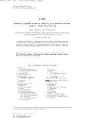
Second graphN(1/n,1/n) vs N(0,1/n); n=100000.0 0.2 0.4 0.6 0.8 1.0N(0,1/n)N(1/n,1/n)•• ••••••••••••••••-3 -2 -1 0 1 2 3N(1/n,1/n) vs N(0,1/n); n=100000.0 0.2 0.4 0.6 0.8 1.0N(0,1/n)N(1/n,1/n)•-0.03 -0.02 -0.01 0.0 0.01 0.02 0.03Richard Lockhart (Simon Fraser University) STAT 830 Convergence in Distribution STAT 830 — Fall 2011 9 / 31

Scaling mattersMultiply both X n and Y n by n 1/2 and let X ∼ N(0,1). Then√ nXn ∼ N(n −1/2 ,1) and √ nY n ∼ N(0,1).Use characteristic functions to prove that both √ nX n and √ nY nconverge to N(0,1) in distribution.If you now let X n ∼ N(n −1/2 ,1/n) and Y n ∼ N(0,1/n) then againboth X n and Y n converge to 0 in distribution.If you multiply X n and Y n in the previous point by n 1/2 thenn 1/2 X n ∼ N(1,1) and n 1/2 Y n ∼ N(0,1) so that n 1/2 X n and n 1/2 Y nare not close together in distribution.You can check that 2 −n → 0 in distribution.Richard Lockhart (Simon Fraser University) STAT 830 Convergence in Distribution STAT 830 — Fall 2011 10 / 31

Third graphN(1/sqrt(n),1/n) vs N(0,1/n); n=100000.0 0.2 0.4 0.6 0.8 1.0N(0,1/n)N(1/sqrt(n),1/n)•• ••••••••••••••••-3 -2 -1 0 1 2 3N(1/sqrt(n),1/n) vs N(0,1/n); n=100000.0 0.2 0.4 0.6 0.8 1.0N(0,1/n)N(1/sqrt(n),1/n)•-0.03 -0.02 -0.01 0.0 0.01 0.02 0.03Richard Lockhart (Simon Fraser University) STAT 830 Convergence in Distribution STAT 830 — Fall 2011 11 / 31

SummaryTo derive approximate distributions:Show sequence of rvs X n converges to some X.The limit distribution (i.e. dstbn of X) should be non-trivial, like sayN(0,1).Don’t say: X n is approximately N(1/n,1/n).Do say: n 1/2 (X n −1/n) converges to N(0,1) in distribution.Richard Lockhart (Simon Fraser University) STAT 830 Convergence in Distribution STAT 830 — Fall 2011 12 / 31

The Central Limit Theorem pp 77–79TheoremIf X 1 ,X 2 ,··· are iid with mean 0 and variance 1 then n 1/2¯X converges indistribution to N(0,1). That is,P(n 1/2¯X ≤ x) →1√2π∫ x−∞e −y2 /2 dy .Richard Lockhart (Simon Fraser University) STAT 830 Convergence in Distribution STAT 830 — Fall 2011 13 / 31

Proof of CLTAs beforeE(e itn1/2¯X) → e −t2 /2 .This is the characteristic function of N(0,1) so we are done by ourtheorem.This is the worst sort of mathematics – much beloved of statisticians– reduce proof of one theorem to proof of much harder theorem.Then let someone else prove that.Richard Lockhart (Simon Fraser University) STAT 830 Convergence in Distribution STAT 830 — Fall 2011 14 / 31

Edgeworth expansionsIn fact if γ = E(X 3 ) thenφ(t) ≈ 1−t 2 /2−iγt 3 /6+···keeping one more term.Thenlog(φ(t)) = log(1+u)whereu = −t 2 /2−iγt 3 /6+··· .Use log(1+u) = u −u 2 /2+··· to getlog(φ(t)) ≈ [−t 2 /2−iγt 3 /6+···]−[···] 2 /2+···which rearranged islog(φ(t)) ≈ −t 2 /2−iγt 3 /6+··· .Richard Lockhart (Simon Fraser University) STAT 830 Convergence in Distribution STAT 830 — Fall 2011 15 / 31

Edgeworth ExpansionsNow apply this calculation tolog(φ T (t)) ≈ −t 2 /2−iE(T 3 )t 3 /6+··· .Remember E(T 3 ) = γ/ √ n and exponentiate to getφ T (t) ≈ e −t2 /2 exp{−iγt 3 /(6 √ n)+···}.You can do a Taylor expansion of the second exponential around 0because of the square root of n and getφ T (t) ≈ e −t2 /2 (1−iγt 3 /(6 √ n))neglecting higher order terms.This approximation to the characteristic function of T can beinverted to get an Edgeworth approximation to the density (ordistribution) of T which looks likef T (x) ≈ 1 √2πe −x2 /2 [1−γ(x 3 −3x)/(6 √ n)+···].Richard Lockhart (Simon Fraser University) STAT 830 Convergence in Distribution STAT 830 — Fall 2011 16 / 31

RemarksThe error using the central limit theorem to approximate a density ora probability is proportional to n −1/2 .This is improved to n −1 for symmetric densities for which γ = 0.These expansions are asymptotic.This means that the series indicated by ··· usually does not converge.When n = 25 it may help to take the second term but get worse ifyou include the third or fourth or more.You can integrate the expansion above for the density to get anapproximation for the cdf.Richard Lockhart (Simon Fraser University) STAT 830 Convergence in Distribution STAT 830 — Fall 2011 17 / 31

Multivariate convergence in distributionDef’n: X n ∈ R p converges in distribution to X ∈ R p ifE(g(X n )) → E(g(X))for each bounded continuous real valued function g on R p .This is equivalent to either of◮ Cramér Wold Device: a t X n converges in distribution to a t X for eacha ∈ R p . or◮ Convergence of characteristic functions:for each a ∈ R p .E(e iat X n) → E(e iatX )Richard Lockhart (Simon Fraser University) STAT 830 Convergence in Distribution STAT 830 — Fall 2011 18 / 31

Extensions of the CLT1 Y 1 ,Y 2 ,··· iid in R p , mean µ, variance covariance Σ thenn 1/2 (Ȳ −µ) converges in distribution to MVN(0,Σ).2 Lyapunov CLT: for each n X n1 ,...,X nn independent rvs withE(X ni ) = 0 Var( ∑ iX ni ) = 1∑E(|Xni | 3 ) → 0then ∑ i X ni converges to N(0,1).3 Lindeberg CLT: 1st two conds of Lyapunov and∑E(X2ni 1(|X ni | > ǫ)) → 0each ǫ > 0. Then ∑ i X ni converges in distribution to N(0,1).(Lyapunov’s condition implies Lindeberg’s.)4 Non-independent rvs: m-dependent CLT, martingale CLT, CLT formixing processes.5 Not sums: Slutsky’s theorem, δ method.Richard Lockhart (Simon Fraser University) STAT 830 Convergence in Distribution STAT 830 — Fall 2011 19 / 31

Slutsky’s Theorem p 75TheoremIf X n converges in distribution to X and Y n converges in distribution (or inprobability) to c, a constant, then X n +Y n converges in distribution toX +c. More generally, if f(x,y) is continuous then f(X n ,Y n ) ⇒ f(X,c).Warning: the hypothesis that the limit of Y n be constant is essential.Richard Lockhart (Simon Fraser University) STAT 830 Convergence in Distribution STAT 830 — Fall 2011 20 / 31

The delta method pp 79-80, 131–135TheoremSuppose:Sequence Y n of rvs converges to some y, a constant.X n = a n (Y n −y) then X n converges in distribution to some randomvariable X.f is differentiable ftn on range of Y n .Then a n (f(Y n )−f(y)) converges in distribution to f ′ (y)X.If X n ∈ R p and f : R p ↦→ R q then f ′ is q ×p matrix of first derivatives ofcomponents of f.Richard Lockhart (Simon Fraser University) STAT 830 Convergence in Distribution STAT 830 — Fall 2011 21 / 31

ExampleSuppose X 1 ,...,X n are a sample from a population with mean µ,variance σ 2 , and third and fourth central moments µ 3 and µ 4 .Thenn 1/2 (s 2 −σ 2 ) ⇒ N(0,µ 4 −σ 4 )where ⇒ is notation for convergence in distribution.For simplicity I define s 2 = X 2 − ¯X 2 .Richard Lockhart (Simon Fraser University) STAT 830 Convergence in Distribution STAT 830 — Fall 2011 22 / 31

How to apply δ method1 Write statistic as a function of averages:◮ DefineW i =[ ]X2i.X i◮ See that [X2¯W n =]X◮ Definef(x 1 ,x 2 ) = x 1 −x 2 2◮ See that s 2 = f( ¯W n ).2 Compute mean of your averages:[ ] [µ W ≡ E( ¯W E(X2n ) = i) µ=2 +σ 2E(X i ) µ].3 In δ method theorem take Y n = ¯W n and y = E(Y n ).Richard Lockhart (Simon Fraser University) STAT 830 Convergence in Distribution STAT 830 — Fall 2011 23 / 31

Delta Method Continues7 Take a n = n 1/2 .8 Use central limit theorem:n 1/2 (Y n −y) ⇒ MVN(0,Σ)where Σ = Var(W i ).9 To compute Σ take expected value of(W −µ W )(W −µ W ) tThere are 4 entries in this matrix. Top left entry is(X 2 −µ 2 −σ 2 ) 2This has expectation:E { (X 2 −µ 2 −σ 2 ) 2} = E(X 4 )−(µ 2 +σ 2 ) 2 .Richard Lockhart (Simon Fraser University) STAT 830 Convergence in Distribution STAT 830 — Fall 2011 24 / 31

Delta Method ContinuesUsing binomial expansion:E(X 4 ) = E{(X −µ+µ) 4 }= µ 4 +4µµ 3 +6µ 2 σ 2 +4µ 3 E(X −µ)+µ 4 .So Σ 11 = µ 4 −σ 4 +4µµ 3 +4µ 2 σ 2 .Top right entry is expectation ofwhich isSimilar to 4th moment get(X 2 −µ 2 −σ 2 )(X −µ)E(X 3 )−µE(X 2 )µ 3 +2µσ 2Lower right entry is σ 2 .So [µ4 −σΣ =4 +4µµ 3 +4µ 2 σ 2 µ 3 +2µσ 2 ]µ 3 +2µσ 2 σ 2Richard Lockhart (Simon Fraser University) STAT 830 Convergence in Distribution STAT 830 — Fall 2011 25 / 31

Delta Method Continues7 Compute derivative (gradient) of f: has components (1,−2x 2 ).Evaluate at y = (µ 2 +σ 2 ,µ) to geta t = (1,−2µ).This leads ton 1/2 (s 2 −σ 2 ) ≈ n 1/2 [1,−2µ][X 2 −(µ 2 +σ 2 )¯X −µ]which converges in distribution to(1,−2µ)MVN(0,Σ).This rv is N(0,a t Σa) = N(0,µ 4 −σ 4 ).Richard Lockhart (Simon Fraser University) STAT 830 Convergence in Distribution STAT 830 — Fall 2011 26 / 31

Alternative approachSuppose c is constant. Define Xi ∗ = X i −c.Sample variance of Xi ∗ is same as sample variance of X i .All central moments of Xi ∗ same as for X i so no loss in µ = 0.In this case:[a t µ4 −σ= (1,0) Σ =4 ]µ 3µ 3 σ 2 .Notice thata t Σ = [µ 4 −σ 4 ,µ 3 ] a t Σa = µ 4 −σ 4 .Richard Lockhart (Simon Fraser University) STAT 830 Convergence in Distribution STAT 830 — Fall 2011 27 / 31

Special Case: N(µ,σ 2 )Then µ 3 = 0 and µ 4 = 3σ 4 .Our calculation hasn 1/2 (s 2 −σ 2 ) ⇒ N(0,2σ 4 )You can divide through by σ 2 and getn 1/2 (s 2 /σ 2 −1) ⇒ N(0,2)In fact ns 2 /σ 2 has χ 2 n−1 distribution so usual CLT shows(n−1) −1/2 [ns 2 /σ 2 −(n−1)] ⇒ N(0,2)(using mean of χ 2 1 is 1 and variance is 2).Factor out n to get√ nn−1 n1/2 (s 2 /σ 2 −1)+(n−1) −1/2 ⇒ N(0,2)which is δ method calculation except for some constants.Difference is unimportant: Slutsky’s theorem.Richard Lockhart (Simon Fraser University) STAT 830 Convergence in Distribution STAT 830 — Fall 2011 28 / 31

Example – medianMany, many statistics which are not explicitly functions of averagescan be studied using averages.Later we will analyze MLEs and estimating equations this way.Here is an example which is less obvious.Suppose X 1 ,...,X n are iid cdf F, density f, median m.We study ˆm, the sample median.If n = 2k −1 is odd then ˆm is the kth largest.If n = 2k then there are many potential choices for ˆm between thekth and k +1th largest.I do the case of kth largest.The event ˆm ≤ x is the same as the event that the number of X i ≤ xis at least k.That isP(ˆm ≤ x) = P( ∑ i1(X i ≤ x) ≥ k)Richard Lockhart (Simon Fraser University) STAT 830 Convergence in Distribution STAT 830 — Fall 2011 29 / 31

The medianSoP(ˆm ≤ x) = P( ∑ 1(X i ≤ x) ≥ k)i(= P √n(ˆFn (x)−F(x)) ≥ √ )n(k/n −F(x)) .From Central Limit theorem this is approximately( √n(k/n )−F(x))1−Φ √ .F(x)(1−F(x))Notice k/n → 1/2.Richard Lockhart (Simon Fraser University) STAT 830 Convergence in Distribution STAT 830 — Fall 2011 30 / 31

MedianIf we put x = m+y/ √ n (where m is true median) we findF(x) → F(m) = 1/2.Also √ n(F(x)−1/2) → f(m) where f is density of F (if f exists).SoP( √ n(ˆm −m) ≤ y) → 1−Φ(−2f(m)y)That is,√ n(ˆm −1/2) → N(0,1/(4f 2 (m))).Richard Lockhart (Simon Fraser University) STAT 830 Convergence in Distribution STAT 830 — Fall 2011 31 / 31