Phenomenological models of cavitation erosion kinetics

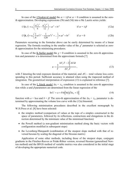
6 International Cavitation Erosion Test Seminar, Sopot, 1-2 June 2000In case of the J.Noskievič model the α = ±β or α = 0 condition is assumed in the zerothapproximation. Developing expressions (5b) and (5d) into a Mc Laurin series yields:2 3 3 4⎛αt α t ⎞3 4U ( k , t) ≈ u ⎜⎟s − = at + bt6 12if α = ±β (12a)⎝⎠⎛ 1 2 3 1 4 5 ⎞ 3 5U ( k , t) = us ⎜ ω t − ω t + ... ⎟ ≈ at + bt if α = 0 (12b)⎝ 6 120 ⎠Parameters occurring in the formulae above can be easily determined by means of a linearregression. The formula resulting in the smaller value of the χ 2 parameter is selected as zerothapproximation for the minimising procedures.In case of the K.Steller model the χ = 0 condition is assumed in the zero-th approximationand parameter κ is determined from the approximate formula [7]∆VTT− 2 ∆Vdt30κ =, (13)T ∆VTwith T denoting the total exposure duration of the material, and ∆V T – total volume loss correspondingto this period. Sufficient accuracy is attained when using the trapezoid method ofintegration. The geometrical interpretation of expression (13) is explained in reference [7].In case of the L.Sitnik model ∆t 0 = τ inc condition is assumed in the zero-th approximationwhile α and β parameters are determined from the linear regression of the[T(T∫ln U = a+ bln ln t ∆t0+ 1)] (14)function with a = lnα and b = β. The zero-th approximation of the ∆t 0 = τ inc parameter is determinedby approximating the volume loss curve with the (12a) binomial.The following minimisation procedures described in the excellent monograph byW.H.Press et al. [8] have been selected:• the simplex method (comparison of values at the tops of a simplex constructed in thespace of parameters, followed by its reflections, contractions and elongations in the directiondetermined by the minimum value of the minimised function)• the Powell method (a non-gradient minimisation method along the basic vectors withconfiguration modified in subsequent steps)• the Levenberg-Marquardt (combination of the steepest slope method with that of reversedhessian by scaling the diagonal of the Hessian matrix)Application of some other methods, including those of the steepest slope, conjugategradients in the Fletcher-Reeves or Polak-Ribier version, reversed Hessian (generalised Newtonmethod) and the BFGS method of variable metrics was also considered in the initial stageof developing the appropriate numerical code.