Phenomenological models of cavitation erosion kinetics

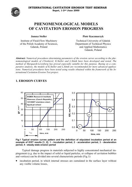
INTERNATIONAL CAVITATION EROSION TEST SEMINARSopot, 1-2 nd June 2000PHENOMENOLOGICAL MODELSOF CAVITATION EROSION PROGRESSJanusz StellerInstitute of Fluid-Flow Machineryof the Polish Academy of Sciences,Gdansk, PolandPiotr KaczmarzykTechnical University of GdańskDepartment of Technical Physicsand Applied MathematicsGdansk, PolandAbstract: Numerical procedures determining parameters of the erosion curves according to the phenomenologicalmodels of J.Noskievič, K.Steller and L.Sitnik have been developed and tested. Themethod of Marquardt-Levenberg has proved especially suitable for this purpose. Basing on a comparativeanalysis, the models of K.Steller and L.Sitnik are recommended for more advanced applications.Numerical procedures have been tested using results obtained within the framework of the InternationalCavitation Erosion Test project.1. EROSION CURVES600.5V, mm 350403020SIGMA Research InstituteOlomouc (Czech Republic),1H18N9T stainless steel,liquid jet wheelIER, mm 3 /min0.40.30.2234100.100 50 100 150 200 2500.010 50 100 150 200 250τ inctime, mintime, minFig.1 Typical erosion curves pattern and the definition of stipulated incubation period at anexample of ICET results [1, 2]; 1 - incubation period, 2 - acceleration period, 3 - decelerationperiod, 4 - steady state erosion periodTypical damage progress in materials subjected to highly concentrated mechanical impingement(e.g. due to the impact of solid or liquid particles, or collapse of cavitation bubblesand vortices) can be divided into several characteristic periods (Fig.1):• incubation period, in which internal stresses are cumulated in the surface layer withoutany visible volume losses,

4 International Cavitation Erosion Test Seminar, Sopot, 1-2 June 2000where the expression under the integral sign denotes erosion rate at the surface element uncoveredin the instant T.F.J.Heymann states that realistic erosion curves can be obtained by assuming the f(t)function to vanish in the initial period of exposure (t ≤ T 0 ), and then to be described by athree-parameter logarithmic-normal distribution[ ln( t − T ) − m]21 ⎪⎧−⎪⎫0f () t = exp⎨2 ⎬(2)σ ( t − T0 ) 2π⎪⎩ 2σ⎪⎭For the original surface layer F.J.Heymann proposes to use a distribution with parametersdifferent from those applied for the subsequent layers. However, there are no hints on themethod of their determination to be found in reference [4].Later on, J.Noskievič [5] and K.Steller [6] proposed models of erosion kinetics referringdirectly to the erosion curve pattern.J.Noskievič has noticed that the instantaneous erosion rate curve, IER =IER(t) remindsthat of damped harmonic oscillator motion. The equation of motion of such an oscillator canbe written asd2( IER) d( IER)dt22+ 2α + β IER = I . (3)dtwith α and β denoting coefficients responsible for material properties (α - work-hardeningcapability, β - cavitation resistance), and I - parameter characterising intensity of cavitationerosive activity (I = const). By assuming erosion rate and its first derivative to vanish at thebeginning of the process, the solution of equation (3) can be written down as−κtκt[( α −κ) e − ( α + κ ) e ]−αt⎧ e⎪vs+ vs⎪2κ−αt⎪vs− vs( 1+α2t)eIER()t = ⎨⎪ ⎛ α ⎞vs− vs⎜cosωt− sinωt⎟e⎪ ⎝ ω ⎠⎪⎩vs− vscosωt−αtififififα > βα = ± βα < βα = 0andα ≠ 0, (4)2 22where κ = α − β and ω = β −α2 , whence the volume loss curve is given by:∆V= vs−αt⎡ α e ⎛α+ κ kt α −κ−kt⎞⎤⎢t− 2 + ⎜ e − e ⎟⎥⎣ β 2if ⏐α⏐ > β (5a)2κ⎝α−κα + κ ⎠⎦∆ V= vs⎡ 2 ⎛ 2 ⎞⎢t− + ⎜t+ ⎟e⎣ α ⎝ α ⎠−αt⎤⎥⎦if α =±β(5b)⎧ α α t ⎡⎛⎞⎤⎫−αα ω∆V = vs⎨t− 2 2+ 2e ⎢⎜− ⎟ sin ωt+2 cosωt⎣⎝⎠⎥⎬,⎩ β β ω α⎦⎭if ⏐α ⏐< β and α ≠ 0 (5c)⎞⎜1∆V= v − s t ω t ⎟⎝ ω sin ,⎠if α = 0 (5d)

J.Steller, P.Kaczmarzyk: Phenomenological models of cavitation erosion progress. 5The formula proposed by K.Steller is based on the notion of cavitation resistance R cav ,clearly linked to that of A.P.Thiruvengadam's erosion strength [7] and defined by the equation:Pt = R cav ∆V (6)where P is the power used to erode the material subject to cavitation impingement. Cavitationis assumed a continuous process (proceeding at variable speed) resulting in the change of bothmaterial surface and its internal structure, responsible for cavitation resistance. Cavitationresistance dependence on duration of cavitation impingement is assumed to be described byan exponentially decreasing functionThe formula derivedRcav( 1+χ )−κtχ + e=1 R 0χ +Pt2 1≈σ∆V=−κt2R0( χ + e )( + χ )EPt−κt( χ + e )shows clear dependence of the volume loss curve ∆V = ∆V(t) on some basic material parameters(modulus of elasticity E and ultimate stress values σ), χ factor determining the ratio ofultimate and initial cavitation resistance (equation (7)), κ parameter defining the speed ofcavitation resistance decrease in course of the process and power P used to erode the material.In mid eighties L.Sitnik [8] assumed the time interval ∆t between removal of the consecutiveparticles from the material surface to be a random function with a three-parameterlogarithmic-natural distribution functionThe volume loss curve derived takes the formFpβ p{ }( ∆t) = 1 − − α [ ln ( ∆t∆t0 + 1)]p(7)(8)exp . (9)β p[ ( t ∆t∆V= α ∆Vln 1)]p0 0 +with ∆V 0 denoting certain characteristic volume value. The α p parameter is characteristic forthe intensity of erosive action of the phenomenon. It is worthwhile to notice that the model isa simplified version of the F.J.Heymann model.(10)3. DETERMINING THE VOLUME LOSS CURVE PARAMETERSACCORDING TO THE SELECTED MODELSOF CAVITATION EROSION KINETICSThe least squares method has been adopted in order to determine the volume loss parametersaccording to selected models. The task can be reduced to that of minimising the expression2[=∑α∆V−χ ( k)U kjjj( , t )]with α j denoting the weight coefficient, U( . , t) - a function describing erosion progress accordingto the model selected, and k - a set (vector) of parameters to be determined by meansof the minimising procedure.During calculations of that kind particular attention should be brought to an appropriateselection of the zero-th approximation.j2,(11)

6 International Cavitation Erosion Test Seminar, Sopot, 1-2 June 2000In case of the J.Noskievič model the α = ±β or α = 0 condition is assumed in the zerothapproximation. Developing expressions (5b) and (5d) into a Mc Laurin series yields:2 3 3 4⎛αt α t ⎞3 4U ( k , t) ≈ u ⎜⎟s − = at + bt6 12if α = ±β (12a)⎝⎠⎛ 1 2 3 1 4 5 ⎞ 3 5U ( k , t) = us ⎜ ω t − ω t + ... ⎟ ≈ at + bt if α = 0 (12b)⎝ 6 120 ⎠Parameters occurring in the formulae above can be easily determined by means of a linearregression. The formula resulting in the smaller value of the χ 2 parameter is selected as zerothapproximation for the minimising procedures.In case of the K.Steller model the χ = 0 condition is assumed in the zero-th approximationand parameter κ is determined from the approximate formula [7]∆VTT− 2 ∆Vdt30κ =, (13)T ∆VTwith T denoting the total exposure duration of the material, and ∆V T – total volume loss correspondingto this period. Sufficient accuracy is attained when using the trapezoid method ofintegration. The geometrical interpretation of expression (13) is explained in reference [7].In case of the L.Sitnik model ∆t 0 = τ inc condition is assumed in the zero-th approximationwhile α and β parameters are determined from the linear regression of the[T(T∫ln U = a+ bln ln t ∆t0+ 1)] (14)function with a = lnα and b = β. The zero-th approximation of the ∆t 0 = τ inc parameter is determinedby approximating the volume loss curve with the (12a) binomial.The following minimisation procedures described in the excellent monograph byW.H.Press et al. [8] have been selected:• the simplex method (comparison of values at the tops of a simplex constructed in thespace of parameters, followed by its reflections, contractions and elongations in the directiondetermined by the minimum value of the minimised function)• the Powell method (a non-gradient minimisation method along the basic vectors withconfiguration modified in subsequent steps)• the Levenberg-Marquardt (combination of the steepest slope method with that of reversedhessian by scaling the diagonal of the Hessian matrix)Application of some other methods, including those of the steepest slope, conjugategradients in the Fletcher-Reeves or Polak-Ribier version, reversed Hessian (generalised Newtonmethod) and the BFGS method of variable metrics was also considered in the initial stageof developing the appropriate numerical code.

J.Steller, P.Kaczmarzyk: Phenomenological models of cavitation erosion progress. 74. NUMERICAL CODE TO CALCULATE PARAMETERSOF EROSION CURVESAND THE ANALYSIS OF OBTAINED RESULTSA computer code APROX [9] has been developed in the Borland Pascal language in orderto accomplish the necessary calculations. The code enables approximation of mass, volumeand mean depth of penetration curves following the models described in section 2, usingone of the above mentioned minimisation methods. The curves of instantaneous and cumulativeerosion rate and basic single-number parameters are also determined. In case of severalspecimens the code determines also the averaged curves and parameters. A hard copy of thecomputer screen, taken during processing of the E04 data at the IMP PAN rotating disk canbe seen in Fig.4.Fig.4 A hard copy of the computer screen, taken during processing the E04 dataThe analysis conducted has proved very good convergence of all the methods in casethe process under consideration covers also the period of steady or quasi-steady damage rate(Fig.5a).The evident superiority of the simplex and Levenberg-Marquardt methods over that ofPowell was stated already in the early stage of analysis. Currently, no problems occur whencalculating the erosion curves according to the models of K.Steller and L.Sitnik. Calculationby means of the simplex method does not always end in global minimisation of formula (11).

8 International Cavitation Erosion Test Seminar, Sopot, 1-2 June 2000∆V, mm 3∆V, mm 320018016014012010080604020IMP PAN (RD) 1H18N9TStellerNoskievic, Sitnik00 200 400 600 800 1000 12005040302010Stellerczas, minIMP PAN (RD) 1H18N9TNoskievicSitnik00 100 200 300 400 500czas, minFig.5 Erosion curves obtained at the IMP PAN rotatingdisk facility (the exposure period of 20 h duration isanalysed)∆V, mm 35040302010IMP PAN (RD) 1H18N9TSitnikNoskievicSteller00 100 200 300 400czas, minFig.6 Erosion curves obtained at the IMP PAN rotatingdisk facility (the exposure period of 6 h duration isanalysed)The work on ensuring full reliabilityof calculations according tothe J.Noskievič model is now in progressand is expected to end successfullyin a short time. Neverthelessthe authors are reluctant to recommendit as an element of more sophisticatedalgorithms due to a rathercomplicated form of formula (5),incorporating additionally some periodicalfunctions.No numerical problems havebeen encountered when testing themodel of K.Steller. However, oneshould notice the non-vanishing firstderivative of formula (7) at the beginningof the process, which canresult in improper modelling of theincubation period and improper assessmentof the maximum instantaneouserosion rate (Fig.5b). On theother hand side, if the analysis isconfined to the period precedingattainment of the maximum cumulativeerosion rate (CER max ), the modelcan describe the reality even betterthan the other ones (Fig.6)Following the model ofL.Sitnik, the erosion rate in the initialstage of damage is always equalzero. The curves obtained show avery smooth pattern, hardly dependenton the duration of analysed period.Therefore, under some circumstances,the model can describe materialperformance in the initial damageperiod worse than the other ones.An obvious advantage is the veryfact that the model has been developedbasing on considerations of thestochastic nature of the cavitationerosion phenomenon. Thus, themodel is a continuation of the originalconcept of F.J.Heymann, somehowrelated to the contemporarymethods of modelling the fatiguephenomena [11].

J.Steller, P.Kaczmarzyk: Phenomenological models of cavitation erosion progress. 9REFERENCES1. Steller J.: International Cavitation Erosion Test. Preliminary Report. Part I: Coordinator'sReport. IMP PAN Int. Rep. no. 19/19982. Steller J.(ed.): International Cavitation Erosion Test. Preliminary Report. Part II: ExperimentalData. IMP PAN Int. Rep. no. 20/19983. Steller J.: International Cavitation Erosion Test and quantitative assessment of materialresistance to cavitation. Wear, Vol.233-235, December 1999, pp.51-644. Heymann F.J.: On the time dependence of the rate of erosion due to impingement or cavitation.[in:] "Erosion by Cavitation or Impingement", A symposium presented at the 69 thAnnual Meeting, ASTM, Atlantic City, 1966. ASTM Special Technical Publicationno.408, pp.70-1005. Noskievič J.: Dynamics of the cavitation damage, Joint Symposium on Design and Operationof Fluid Machinery, ASCE/IAHR/ASME, Colorado State University, Fort Collins,June 1978, pp.453-4626. Steller K.: Nowa koncepcja oceny odporności materiału na erozję kawitacyjną.Prace IMP, z.76, 1978, s.127-1507. Thiruvengadam A.P.: The concept of erosion strength. Erosion by cavitation or impingement[in:] "Erosion by Cavitation or Impingement", A symposium presented at the 69 thAnnual Meeting, ASTM, Atlantic City, 1966. ASTM Special Technical Publicationno.408, pp.22-358. Sitnik L.: Mathematical description of the cavitation erosion process and its utilizationfor increasing the materials resistance to cavitation. [in:] "Cavitation in Hydraulic Structuresand Turbomachinery". The Joint ASCE/ASME Mechanics Conf., Albuquerque,New Mexico, 1985, pp.21-309. Press W.H., Teukolsky S.A., Vetterling W.T., Flannery B.P.: Numerical Recipes in FOR-TRAN 77. The Art of Scientific Computing. Cambridge University Press, 199210. Kaczmarzyk P.: Kinetics of the cavitation erosion process in view of the InternationalCavitation Erosion Test results (in Polish). MSc Thesis, Faculty of Technical Physicsand Applied Mathematics, Technical University of Gdansk, Gdansk, 2000(under preparation)11. Sobczyk K., Spencer B.F.: Stochastyczne modele zmęczenia materiałów,WNT, Warszawa, 1996AuthorsDr Janusz StellerInstytut Maszyn Przepływowych PANul. Gen. J. Fiszera 1480-952 Gdańsk, Polandphone: +48 58 341 12 71 ext. 139e-mail: steller@imp.pg.gda.plPiotr KaczmarzykPolitechnika GdańskaWydział Fizyki Techniczneji Matematyki Stosowanej,ul. G. Narutowicza 1180-952 Gdańsk, Poland