The boundary-path space of a directed graph - 56th ... - CARMA
The boundary-path space of a directed graph - 56th ... - CARMA
The boundary-path space of a directed graph - 56th ... - CARMA
- No tags were found...

You also want an ePaper? Increase the reach of your titles
YUMPU automatically turns print PDFs into web optimized ePapers that Google loves.
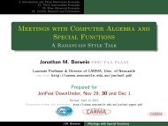
<strong>The</strong> <strong>boundary</strong>-<strong>path</strong> <strong>space</strong> <strong>of</strong> a <strong>directed</strong> <strong>graph</strong>56 th AustMS AGM, BallaratS.B.G. WebsterUniversity <strong>of</strong> Wollongong25 September 2012MODEL / ANALYSE / FORMULATE /ILLUMINATECONNECT:IMIA
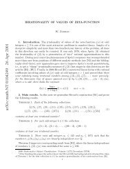
DefinitionA <strong>directed</strong> <strong>graph</strong> E is a set E 0 <strong>of</strong> vertices and a set E 1 <strong>of</strong> <strong>directed</strong>edges, with direction determined by range and source mapsr, s : E 1 → E 0 .ExampleevfwE 0 = {v, w} E 1 = {e, f }s(e) = r(e) = r(f ) = vs(f ) = w
Paths◮ A sequence µ 1 µ 2 µ 3 . . . <strong>of</strong> edges is a <strong>path</strong> if s(µ i ) = r(µ i+1 ) forall i.r(µ)µ 1 µ ns(µ)
Paths◮ A sequence µ 1 µ 2 µ 3 . . . <strong>of</strong> edges is a <strong>path</strong> if s(µ i ) = r(µ i+1 ) forall i.r(µ)µ 1 µ ns(µ)◮ E n = {µ : µ is a <strong>path</strong> with n (possibly = ∞) edges}◮ E ∗ = {µ : µ has finitely many edges}.◮ For V ⊂ E 0 and F ⊂ E ∗ , define VF := F ∩ r −1 (V ).◮ In particular, for v ∈ E 0 , vF = F ∩ r −1 (v).
Graph C ∗ -algebras◮ E ≤n := {µ ∈ E ∗ : |µ| = n, or |µ| < n and s(µ)E 1 = ∅}.◮ <strong>The</strong> <strong>graph</strong> C ∗ -algebra C ∗ (E) is universal for C ∗ -algebrascontaining a Cuntz-Krieger E-family: a family consisting <strong>of</strong>mutually orthogonal projections {s v : v ∈ E 0 } and partialisometries {s µ : µ ∈ E ∗ } such that {s µ : µ ∈ E ≤n } have mutuallyorthogonal ranges for each n ∈ N, and such that1. s ∗ µs µ = s s(µ) ;2. s µ s ν = s µν when s(µ) = r(ν);3. s µ s ∗ µ ≤ s r(µ) ; and4. s v = ∑µ∈vE ≤n s µ s ∗ µ for every v ∈ E 0 and n ∈ N such that|vE ≤n | < ∞.
Diagonal sub-C ∗ -algebra◮ We call D E := C ∗ (s λ s ∗ λ : λ ∈ E ∗ ) the diagonal C ∗ -subalgebra <strong>of</strong>C ∗ (E).◮ It can be deduced from the Cuntz-Krieger relations thatD = span{s λ s ∗ λ : λ ∈ E ∗ }.
Diagonal sub-C ∗ -algebra◮ We call D E := C ∗ (s λ s ∗ λ : λ ∈ E ∗ ) the diagonal C ∗ -subalgebra <strong>of</strong>C ∗ (E).◮ It can be deduced from the Cuntz-Krieger relations thatD = span{s λ s ∗ λ : λ ∈ E ∗ }.◮ For each n ∈ N, {s λ s ∗ λ : λ ∈ E n } are mutually orthogonalprojections.
Diagonal sub-C ∗ -algebra◮ We call D E := C ∗ (s λ s ∗ λ : λ ∈ E ∗ ) the diagonal C ∗ -subalgebra <strong>of</strong>C ∗ (E).◮ It can be deduced from the Cuntz-Krieger relations thatD = span{s λ s ∗ λ : λ ∈ E ∗ }.◮ For each n ∈ N, {s λ s ∗ λ : λ ∈ E n } are mutually orthogonalprojections.◮ Write µ ≼ λ ⇐⇒ λ = µµ ′ . <strong>The</strong>n µ ≼ λ ⇐⇒ s λ s ∗ λ ≤ s µs ∗ µ.
Diagonal sub-C ∗ -algebra◮ We call D E := C ∗ (s λ s ∗ λ : λ ∈ E ∗ ) the diagonal C ∗ -subalgebra <strong>of</strong>C ∗ (E).◮ It can be deduced from the Cuntz-Krieger relations thatD = span{s λ s ∗ λ : λ ∈ E ∗ }.◮ For each n ∈ N, {s λ s ∗ λ : λ ∈ E n } are mutually orthogonalprojections.◮ Write µ ≼ λ ⇐⇒ λ = µµ ′ . <strong>The</strong>n µ ≼ λ ⇐⇒ s λ s ∗ λ ≤ s µs ∗ µ.◮ Denote the spectrum <strong>of</strong> D by ∆ D .
Diagonal sub-C ∗ -algebra◮ We call D E := C ∗ (s λ s ∗ λ : λ ∈ E ∗ ) the diagonal C ∗ -subalgebra <strong>of</strong>C ∗ (E).◮ It can be deduced from the Cuntz-Krieger relations thatD = span{s λ s ∗ λ : λ ∈ E ∗ }.◮ For each n ∈ N, {s λ s ∗ λ : λ ∈ E n } are mutually orthogonalprojections.◮ Write µ ≼ λ ⇐⇒ λ = µµ ′ . <strong>The</strong>n µ ≼ λ ⇐⇒ s λ s ∗ λ ≤ s µs ∗ µ.◮ Denote the spectrum <strong>of</strong> D by ∆ D .<strong>The</strong>n for each φ ∈ ∆ D andµ ≼ λ, we have φ(s λ s ∗ λ ) = 1 =⇒ φ(s µs ∗ µ) = 1.
Diagonal sub-C ∗ -algebra◮ We call D E := C ∗ (s λ s ∗ λ : λ ∈ E ∗ ) the diagonal C ∗ -subalgebra <strong>of</strong>C ∗ (E).◮ It can be deduced from the Cuntz-Krieger relations thatD = span{s λ s ∗ λ : λ ∈ E ∗ }.◮ For each n ∈ N, {s λ s ∗ λ : λ ∈ E n } are mutually orthogonalprojections.◮ Write µ ≼ λ ⇐⇒ λ = µµ ′ . <strong>The</strong>n µ ≼ λ ⇐⇒ s λ s ∗ λ ≤ s µs ∗ µ.◮ Denote the spectrum <strong>of</strong> D by ∆ D .<strong>The</strong>n for each φ ∈ ∆ D andµ ≼ λ, we have φ(s λ s ∗ λ ) = 1 =⇒ φ(s µs ∗ µ) = 1.◮ Hence for each φ ∈ ∆ D , the elements <strong>of</strong> {λ : φ(s λ s ∗ λ ) = 1}determine a <strong>path</strong>.
Boundary Paths◮ <strong>The</strong> <strong>path</strong>s we get turn out to be all infinite <strong>path</strong>s, and all finite<strong>path</strong>s whose source is a singular vertex: elements v ∈ E 0satisfying either◮ vE 1 = ∅, in which case we call v a source; or◮ |vE 1 | = ∞, in which case we call v an infinite receiver.
Boundary Paths◮ <strong>The</strong> <strong>path</strong>s we get turn out to be all infinite <strong>path</strong>s, and all finite<strong>path</strong>s whose source is a singular vertex: elements v ∈ E 0satisfying either◮ vE 1 = ∅, in which case we call v a source; or◮ |vE 1 | = ∞, in which case we call v an infinite receiver.◮ We define the <strong>boundary</strong> <strong>path</strong>s∂E := E ∞ ∪ {µ ∈ E ∗ : s(µ) is singular}.
Boundary Paths◮ <strong>The</strong> <strong>path</strong>s we get turn out to be all infinite <strong>path</strong>s, and all finite<strong>path</strong>s whose source is a singular vertex: elements v ∈ E 0satisfying either◮ vE 1 = ∅, in which case we call v a source; or◮ |vE 1 | = ∞, in which case we call v an infinite receiver.◮ We define the <strong>boundary</strong> <strong>path</strong>s∂E := E ∞ ∪ {µ ∈ E ∗ : s(µ) is singular}.◮ <strong>The</strong> formulah E (x)(s µ s ∗ µ) ={1 if µ ≼ x0 otherwise.uniquely determines a bijection from ∂E onto ∆ D [W].
Topology◮ Following the approach <strong>of</strong> [PW], define α : E ∗ ∪ E ∞ → {0, 1} E ∗by{1 if x = µµ ′α(x)(µ) =0 otherwise.◮ Give E ∗ ∪ E ∞ the initial topology induced by α.
Topology◮ Following the approach <strong>of</strong> [PW], define α : E ∗ ∪ E ∞ → {0, 1} E ∗by{1 if x = µµ ′α(x)(µ) =0 otherwise.◮ Give E ∗ ∪ E ∞ the initial topology induced by α.◮ For µ ∈ E ∗ , define Z(µ) := {µµ ′ ∈ E ∗ ∪ E ∞ }.◮ For G ⊂ E ∗ , we write Z(µ \ G) := Z(µ) \ ⋃ ν∈G Z(ν).◮ <strong>The</strong> cylinder sets {Z(µ \ G) : µ ∈ E ∗ , G ⊂ s(µ)E 1 is finite} are abasis for our topology. [W].
Topology◮ Following the approach <strong>of</strong> [PW], define α : E ∗ ∪ E ∞ → {0, 1} E ∗by{1 if x = µµ ′α(x)(µ) =0 otherwise.◮ Give E ∗ ∪ E ∞ the initial topology induced by α.◮ For µ ∈ E ∗ , define Z(µ) := {µµ ′ ∈ E ∗ ∪ E ∞ }.◮ For G ⊂ E ∗ , we write Z(µ \ G) := Z(µ) \ ⋃ ν∈G Z(ν).◮ <strong>The</strong> cylinder sets {Z(µ \ G) : µ ∈ E ∗ , G ⊂ s(µ)E 1 is finite} are abasis for our topology. [W].◮ With this topology, E ∗ ∪ E ∞ is locally compact and Hausdorff[W].
Boundary Paths◮ Fix a <strong>path</strong> µ ∈ E ∗ with 0 < |s(µ)E 1 | < ∞.◮ <strong>The</strong>n {µ} = Z ( µ \ {s(µ)E 1 } ) an open set.◮ <strong>The</strong>nU := ⋃ {{µ} : µ ∈ E ∗ such that 0 < |s(µ)E 1 | < ∞ }is open.
Boundary Paths◮ Fix a <strong>path</strong> µ ∈ E ∗ with 0 < |s(µ)E 1 | < ∞.◮ <strong>The</strong>n {µ} = Z ( µ \ {s(µ)E 1 } ) an open set.◮ <strong>The</strong>nis open.U := ⋃ {{µ} : µ ∈ E ∗ such that 0 < |s(µ)E 1 | < ∞ }◮ So ∂E = U c is closed in E ∗ ∪ E ∞ , and hence locally compactand Hausdorff.
Boundary Paths◮ Fix a <strong>path</strong> µ ∈ E ∗ with 0 < |s(µ)E 1 | < ∞.◮ <strong>The</strong>n {µ} = Z ( µ \ {s(µ)E 1 } ) an open set.◮ <strong>The</strong>nis open.U := ⋃ {{µ} : µ ∈ E ∗ such that 0 < |s(µ)E 1 | < ∞ }◮ So ∂E = U c is closed in E ∗ ∪ E ∞ , and hence locally compactand Hausdorff.◮ <strong>The</strong> map h E : ∂E → ∆ D is a homeomorphism [W].
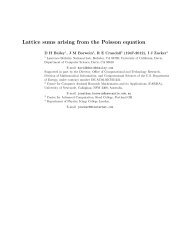
DesingularisationDrinen and Tomforde developed a construction they calleddesingularisation [DT]:◮ Suppose E has some singular vertices. Fix µ ∈ ∂E ∩ E ∗ .◮ If |s(µ)E 1 | = 0, then append on an infinite <strong>path</strong>:µ• •
DesingularisationDrinen and Tomforde developed a construction they calleddesingularisation [DT]:◮ Suppose E has some singular vertices. Fix µ ∈ ∂E ∩ E ∗ .◮ If |s(µ)E 1 | = 0, then append on an infinite <strong>path</strong>:µµ• •becomes• •. . .
DesingularisationDrinen and Tomforde developed a construction they calleddesingularisation [DT]:◮ Suppose E has some singular vertices. Fix µ ∈ ∂E ∩ E ∗ .◮ If |s(µ)E 1 | = 0, then append on an infinite <strong>path</strong>:µµ• •becomes• •◮ If |s(µ)| = ∞, then append an infinite <strong>path</strong>, and distribute theincoming edges along it:•. . .s(µ). . .
DesingularisationDrinen and Tomforde developed a construction they calleddesingularisation [DT]:◮ Suppose E has some singular vertices. Fix µ ∈ ∂E ∩ E ∗ .◮ If |s(µ)E 1 | = 0, then append on an infinite <strong>path</strong>:µµ• •becomes• •◮ If |s(µ)| = ∞, then append an infinite <strong>path</strong>, and distribute theincoming edges along it:•. . .s(µ)becomes•s(µ). . .. . .• • •. . .
Desingularisation◮ Let E be a <strong>directed</strong> <strong>graph</strong>, and F be a Drinen-Tomfordedesingularisation <strong>of</strong> E.◮ This gives a homeomorphism φ ∞ : E 0 F ∞ → ∂E [DT,W].◮ <strong>The</strong>n there exists a full projection p and an isomorphismπ : C ∗ (E) → pC ∗ (F )p [DT].
All together now◮ For each <strong>directed</strong> <strong>graph</strong> E, we have h E : ∂E ∼ = ∆ DE . [W]
All together now◮ For each <strong>directed</strong> <strong>graph</strong> E, we have h E : ∂E ∼ = ∆ DE . [W]◮ Given a desingularisation <strong>of</strong> E, we have φ ∞ : E 0 F ∞ ∼ = ∂E.[DT,W].
All together now◮ For each <strong>directed</strong> <strong>graph</strong> E, we have h E : ∂E ∼ = ∆ DE . [W]◮ Given a desingularisation <strong>of</strong> E, we have φ ∞ : E 0 F ∞ ∼ = ∂E.[DT,W].◮ π induces a homeomorphism π ∗ : ∆ pDF p → ∆ DE [W].
All together now◮ For each <strong>directed</strong> <strong>graph</strong> E, we have h E : ∂E ∼ = ∆ DE . [W]◮ Given a desingularisation <strong>of</strong> E, we have φ ∞ : E 0 F ∞ ∼ = ∂E.[DT,W].◮ π induces a homeomorphism π ∗ : ∆ pDF p → ∆ DE◮ <strong>The</strong>se maps commute [W]:[W].E 0 F ∞φ ∞∂Eη∆ pDF pπ ∗∆ DEh EWhere η is essentially the restriction <strong>of</strong> h Fto <strong>path</strong>s with ranges in E 0 .
References[DT] D. Drinen and M. Tomforde, <strong>The</strong> C ∗ -algebras <strong>of</strong> arbitrary<strong>graph</strong>s, Rocky Mountain J. Math. 35 (2005), 105–135.[PW] A.L.T. Paterson and A.E. Welch, Tychon<strong>of</strong>f’s theorem for locallycompact <strong>space</strong>s and an elementary approach to the topology <strong>of</strong><strong>path</strong> <strong>space</strong>s, Proc. Amer. Math. Soc. 133 (2005), 2761–2770.[W] S.B.G. Webster, <strong>The</strong> <strong>path</strong> <strong>space</strong> <strong>of</strong> a <strong>directed</strong> <strong>graph</strong>, Proc.Amer. Math. Soc., to appear.