Modeling of Bubble Column Reactors: Progress and Limitations

Ind. Eng. Chem. Res. 2005, 44, 5107-51515107Modeling of Bubble Column Reactors: Progress and LimitationsHugo A. Jakobsen,* Håvard Lindborg, and Carlos A. DoraoDepartment of Chemical Engineering, Norwegian University of Science and Technology,NTNU, Sem Sælands vei 4, NO-7491 Trondheim, NorwayBubble columns are widely used for carrying out gas-liquid and gas-liquid-solid reactions ina variety of industrial applications. The dispersion and interfacial heat- and mass-transfer fluxes,which often limit the overall chemical reaction rates, are closely related to the fluid dynamicsof the system through the liquid-gas contact area and the turbulence properties of the flow.There is thus considerable interest, within both academia and industry, to improve the limitedunderstanding of the complex multiphase flow phenomena involved, which is preventing optimalscale-up and design of these reactors. In this paper, the progress reported in the literature duringthe past decade regarding the use of averaged Eulerian multifluid models and computationalfluid dynamics (CFD) to model vertical bubble-driven flows is reviewed. The limiting steps inthe model derivation are the formulation of proper boundary conditions, closure laws determiningturbulent effects, interfacial transfer fluxes, and the bubble coalescence and breakage processes.Examples of both classical and more recent modeling approaches are described, evaluated, anddiscussed. Physical mechanisms and numerical modes creating bubble movement in the radialdirection are outlined. Special emphasis is placed on the population balance modeling of thebubble coalescence and breakage processes in two-phase bubble column reactors. The constitutiverelations used to describe the bubble-bubble and bubble-turbulence interactions, the bubblecoalescence and breakage criteria, and the daughter size distribution models are discussed witha focus on model limitations. The demand for amplified modeling, more accurate and stablenumerical algorithms, and experimental analysis providing data for proper model validation isstressed.1. IntroductionChemical reaction engineering (CRE) has emerged asa methodology that quantifies the interplay betweentransport phenomena and kinetics on a variety of scalesand allows the formulation of quantitative models forvarious measures of reactor performance. The abilityto establish such quantitative links between measuresof reactor performance and input and operating variablesis essential in optimizing the operating conditionsin manufacturing, in determining proper reactor designand scale-up, and in correctly interpreting data inresearch and pilot-plant work.A starting point for reaction engineers is the formulationof a reactor model for which the basis is themicroscale species mass and enthalpy balances. Forpractical applications, the direct solution of these equationsis excessively costly, and simplifications or averagerepresentations are usually introduced.The choice of averages (e.g., global reactor volume,cross-sectional area, or length) over which the balanceequations are integrated (averaged) determines the levelof sophistication of the reactor model. It is very commonin tubular reactors to have flow predominantly in onespatial direction, say, z. The major gradients then occurin that direction. For many cases, then, the crosssectionalaverage values of concentration and temperatureare used instead of the local values. In this way,a one-dimensional dispersion model is obtained. If theconvective transport is completely dominant over the* To whom correspondence should be addressed. E-mail:jakobsen@chemeng.ntnu.no. Tel.: + 47 73594132. Fax: + 4773594080.diffusive transport, the diffusive term can be neglected.The resulting equations are denoted the ideal plug-flowreactor (PFR) model. When the entire reactor can beconsidered to be uniform in both concentration andtemperature (i.e., because of very large dispersioncoefficients), one can neglect gradients in all spatialdirections and integrate the equations globally over allspatial dimensions (assuming convective flows at theboundaries), leading to the ideal reactor model of thecontinuous stirred tank reactor (CSTR). For morecomplex flow patterns, more elaborated and completemodels are required where the flow fields are describedvia the solution of the Navier-Stokes equations. Theunderstanding of the complex flow phenomena involvedas well as the solution of these vector equations makethe problem much more difficult to analyze within theconstraint of reasonable costs and efforts. In these cases,the full set of governing equations can be averaged overlocal but finite spatial and temporal scales to obtainformulations that are solved with feasible space andtime resolutions. The latter type of models can also beobtained using other local averaging procedures aswell.Two-phase and slurry bubble columns are widely usedin the chemical and biochemical industries for carryingout gas-liquid and gas-liquid-solid (catalytic) reactionprocesses. 1-6 The historical development of bubblecolumn modeling was discussed in a recent paper byDudukovic. 4 In the past, the axial dispersion model wascommonly applied for both the gas and liquid (slurry)phases in bubble columns. 2,7 The balance equationsdetermining the liquid- (slurry-) phase axial dispersionmodel can be written as10.1021/ie049447x CCC: $30.25 © 2005 American Chemical SocietyPublished on Web 01/20/2005

5108 Ind. Eng. Chem. Res., Vol. 44, No. 14, 2005d(F L v S z,L ω i,L )anddz) ɛ L F L D z,Ld 2 ω i,Ldz 2/+ k L a(F L,i-F L,i ) +ɛ L∑γ i,r R L,r (1)rdT L d 2 T LSF L C P,L v z,Ldz ) ɛ L λ z,L + h dz 2 W a W (T W - T L ) +ɛ L∑(-∆H r )R r,L (2)rIn these balance equations, all terms should bedescribed at the same level of accuracy. It certainly doesnot pay to have the finest description of one term in thebalance equations if the others can only be very crudelydescribed. Current demands for increased selectivityand volumetric productivity require more precise reactormodels and also force reactor operation to churn turbulentflow, which, to a great extent, is unchartedterritory. An improvement in accuracy and a moredetailed description of the molecular-scale events describingthe rate of generation term in the heat- andmass-balance equations has, in turn, pushed forward aneed for a more detailed description of the transportterms (i.e., in the convection/advection and dispersion/conduction terms in the basic mass and heat balances).Experimental evidence shows that the liquid axialvelocity is far from being flat and independent of theradial space coordinate, 2 and the use of a cross-sectionalaverage velocity variable seems not to be sufficient. Theback-mixing induced by the global liquid flow patternhas commonly been taken into account by adjusting theaxial dispersion coefficient accordingly. However, eventhough (slurry) bubble column performance often canbe fitted with an axial dispersion model, decades ofresearch have failed to produce a predictive equationfor the axial dispersion coefficient.Hence, research is in progress to quantify theseparameters based on first principles (e.g., see Jakobsenet al., 8 Joshi, 9 Rafique et al., 10 and references therein).However, despite their simple construction, the fluiddynamics observed in these columns is very complex.Even though CFD modeling concepts have been extendedover the past two decades in accordance withthe rapid progress in computer performance, the modelcomplexity required to resolve all of the importantphenomena in these systems is still not feasible withinreasonable time limits. The multifluid model is foundto represent a tradeoff between accuracy and computationalefforts for practical applications.Unfortunately, the present models are still on a levelaiming at reasonable solutions with several modelparameters tuned to known flow fields. For predictivepurposes, these models are hardly able to predictunknown flow fields with a reasonable degree of accuracy.It appears that CFD evaluations of bubblecolumns by use of multidimensional multifluid modelsstill have very limited inherent capabilities to fullyreplace the empirical-based analyses (i.e., in the frameworkof axial dispersion models) in use today. 11,12 Aftertwo decades of performing fluid dynamic modeling ofbubble columns, it has been realized that there iscertainly a limit to how accurate one will be able informulating closure laws using the Eulerian framework.A severe problem is that, although the Eulerian modelingprospects are not outstanding, no other conceptsavailable are favorable for the purpose of predictingbubble column flows. A more relevant question is thus:What can be achieved by adopting the Eulerian multifluidmodeling framework for the purpose of describingchemical processes operated in bubble column reactors?The authors intend the following summary to providecertain guidelines for the discussion but, of course, nocomplete answer to this question.Fluid Dynamic Modeling. Considering modeling infurther detail, the general picture from the literatureis that the forces acting on the dispersed phase are 8inertia, gravity, buoyancy, viscous, pressure, lift, wall,turbulent stress, turbulent dispersion, steady-drag, andadded-mass forces. In the latest papers (i.e., publishedafter the review by Jakobsen et al. 8 ) performing 3Dsimulations, the force balances in vertical bubbly flowswere found to be determined by only a few of theseforces. The axial component of the momentum equationfor the gas phase is dominated by the pressure andsteady-drag forces only, indicating that algebraic slipmodels might be sufficient, 13-15 whereas most multifluidmodels also retain the inertia and gravity (buoyancy)terms. The axial momentum balance for the liquid phaseconsiders the inertia, turbulent stress, pressure, steadydrag,and gravity forces. Only pressure and buoyancyforces are acting on a motionless bubble in a liquid atrest. In the radial and azimuthal directions, the forcebalances generally includes the steady-drag force, i.e.,a force that opposes motion, whereas the pertinentforces causing motion are more difficult to define. In avery short inlet zone, the wall friction is likely to inducea radial pressure gradient that pushes the gas bubblesaway from the wall, whereas a few column diametersabove the inlet, the radial pressure gradient vanishes.It is still an open question whether this pressuregradient is sufficient to determine the phase distributionsobserved in these systems. It is expected that thepresence of the wall induce forces that act on thedispersed particles farther from the inlet, but there isno general acceptance on the physical mechanisms andformulations of these forces. It is also a matter ofdiscussion whether this wall effect should be taken intoaccount indirectly through the liquid wall friction or,in view of the model averaging performed, directly as aforce in the gas-phase equations. The bulk lift forces donot induce any radial bubble movement without aninitial velocity gradient, so other forces are importantin the initial phase of the flow pattern development. Inthe generalized drag formulation, the interfacial couplingis expressed as a linear sum of independent forces;this point of view is probably not valid when the voidfraction exceeds a few percent. Moreover, the parametrizationsused for the coefficients occurring in theinterfacial closures vary significantly, especially athigher void fractions. Single-particle drag, added-mass,and lift coefficients are most frequently used, whereasswarm corrections have been included in some codes.For higher void fractions, other rather empirical correctionshave been introduced as well. 16The flow of the continuous phase is considered to beinitiated by a balance between the interfacial particlefluidcoupling and wall friction forces, whereas the fluidphaseturbulence damps the macroscale dynamics of thebubble swarms, thereby smoothing the velocity andvolume fraction fields. Temporal instabilities induced

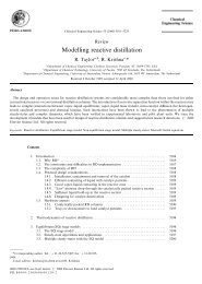
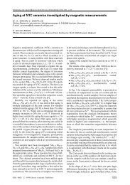
Ind. Eng. Chem. Res., Vol. 44, No. 14, 2005 5109Figure 1. Classification of regions accounting for the macroscopic flow structures: left, 2D bubble column; 21 right, 3D bubble column. 23by the fluid inertia terms create inhomogeneities in theforce balances. Unfortunately, proper modeling of turbulenceis still one of the main open issues in gas-liquidbubbly flows, and this flow property can significantlyaffect both the stresses and the bubble dispersion. 15It was shown by Svendsen et al., 17 among others, thatthe time-averaged experimental data on the flow patternin cylindrical bubble columns apparently becomesclose to axisymmetric. Fair agreement between experimentaland simulated results are generally obtained forthe steady velocity fields in both phases, whereas thesteady phase distribution is still a problem. Therefore,it was anticipated that 2D axisymmetric simulationswould capture the pertinent time-averaged flow patternneeded for the analysis of many (not all) mechanismsof interest for chemical engineers. Sanyal et al. 18 andKrishna and van Baten, 19 for example, stated that 2Dmodels provide good engineering descriptions, althoughthey are not able to capture the high-frequency unsteadybehavior of the flow, and can be used for approximatelypredicting the low-frequency time-averaged flow andvoid patterns in bubble columns.The early 2D steady-state model proposed by Jakobsen20 was able to capture the global flow pattern fairlywell, provided that a large negative lift force wasincluded. However, after the first elaborated experimentalstudies on 2D rectangular bubble columns werepublished by Tzeng et al. 21 and Lin et al., 22 it wascommonly accepted that time-average computationscannot provide a rational explanation of the transportprocesses of mass, momentum, and energy between thebubbles and liquid. The experimental data obtainedwere analyzed, and sketches of their interpretations ofthe dynamic flow patterns in both 2D and 3D columnswere given, as shown in Figure 1. It was concluded thata proper bubble column model should consider thetransient or instantaneous flow behavior. A few yearslater, Sokolichin and Eigenberger, 24 Sokolichin et al., 25and Sokolichin and Eigenberger 26 claimed that dynamic3D models were needed to provide sufficient representationsof the high-frequency unsteady behavior of theseflows. Very different dynamic flow patterns can resultin quantitatively similar long-time-averaged flow profiles.This limits the use of long-time-averaged flowprofiles for validation of bubbly flow models. van denFigure 2. Lateral movement of the bubble hose in a flat bubblecolumn. 28 Reprinted with permission from Elsevier.Akker, 12 among others, questioned the early turbulencemodeling performed (or rather the lack of any) in thesestudies and argued that the apparently realistic simulationsof the transient flow characteristics could benumerical modes rather than physical ones (see alsoSokolichin et al. 15 ). Insufficiently fine grids might havebeen used in the simulations, resulting in numericalinstabilities that could be erroneously interpreted asphysical ones. However, after the observation of Sokolichinand Eigenberger was reported, intensive focus onthese instability issues were made, mainly by researchersfrom the fluid dynamics community. The experimentaldata provided by Becker et al. 27,28 (see Figure2) still serve as a benchmark test and are often usedfor validation of dynamic flow models. The numericalinvestigations were restricted to bubbly flow hydrodynamics(i.e., no reactive systems were analyzed),where additional simplifications were made: isothermalconditions, no interfacial mass transfer, constant liquiddensity, gas density constant or depending on localpressure as described by the ideal gas law, and nobubble coalescence and breakage.However, after the dynamic flow structures wereobserved, bubble columns have generally been simu-

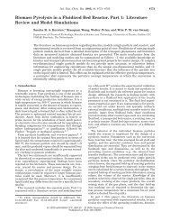
5110 Ind. Eng. Chem. Res., Vol. 44, No. 14, 2005lated using either 2D or 3D dynamic models for bothcylindrical 18,29-36 and rectangular 2D and 3D columngeometries. 14,15,34,35,37-43 The gas is introduced adoptingboth uniform and localized feedings at the bottom of thecolumn. The modeling of systems uniformly gassed atthe bottom is more difficult than the modeling of partlyaerated ones. Simulating systems with continuous liquidflow is also more difficult than keeping the liquid inbatch mode. Finally, it is also noted that the differentresearch groups applied both commercial codes(e.g., CFX, FLUENT, PHOENICS, CFDLIB, ASTRID,NPHASE) and several in-house codes in which theinherent choices of numerical methods, discretizations,grid arrangements, and boundary implementations varyquite widely. These numerical differences alter thesolutions to some extent, so it should not be expectedthat the corresponding simulations will provide identicalresults. An open and unified research code available forall research groups could assist by eliminating anymisinterpretations of numerical modes as physicalmechanisms and visa versa.Considering the interfacial and turbulent closures forvertical bubble-driven flows, no extensive progress hasbeen observed in the later publications. However, twodiverging modeling trends seem to emerge because ofthe lack of understanding of the phenomena involvedand how to deal with these phenomena within anaverage modeling framework. One group of papersconsiders only phenomena that can be validated withthe existing experimental techniques and thus containsa minimum number of terms and effects. Papers in theother group include a large number of weakly foundedtheoretical hypothesis and relations intended to resolvethe missing mechanisms.Steady-State or Dynamic Simulations, Closures,and Numerical Grid Arrangements. Not only dynamicmodels have been adopted investigating thesephenomena. Lopez de Bertodano, 44 for example, used a3D steady finite-volume method (FVM) (PHOENICS)with a staggered grid arrangement to simulate turbulentbubbly two-phase flow in a triangular duct. In thisstudy, the lift, turbulent dispersion, and steady-dragforces were assumed to be dominant. Standard literatureexpressions were adopted for the drag and liftforces, whereas a crude model for the turbulent dispersionforce was developed. An extended k-ɛ model,considering bubble-induced turbulence, was also developedfor the liquid-phase turbulence. It was proposedthat the shear-induced turbulence and the bubbleinducedturbulence could be superimposed. The lift forcewas found to be essential to reproducing the experimentallyobserved wall void peaks satisfactorily. Anglartet al. 45 adopted many of the same closures withina 2D steady version of the same code (PHOENICS),predicting low-void bubbly flow between two parallelplates. They found satisfactory agreement with experimentaldata when applying drag, added-mass, lift, wall(lubrication), and turbulent diffusion forces in theirstudy. The extended k-ɛ model of Lopez de Bertodano 44was applied for the liquid-phase turbulence. In a morerecent paper, Antal et al. 46 adopted very similar closuresfor 3D steady-state bubble column simulations using theNPHASE code. The NPHASE CMFD code employs anFVM on a collocated grid. A three-field multifluid modelformulation was used to simulate two-phase flow in abubble column operating in the churn-turbulent flowregime. The gas phase was subdivided into two fields(i.e., small and large bubbles) to more accuratelydescribe the interfacial momentum-transfer fluxes. Thethird field was used for the liquid phase. The modelresults were validated against a few time-averaged datasets for the liquid axial velocity and the gas volumefraction. Global flow patterns for all three fields and theoverall gas volume fractions were shown. The simulationswere in fair agreement with the experimentalobservations. Using a 2D in-house FVM code with astaggered grid arrangement, Dhotre and Joshi 47 predictedthe flow pattern, pressure drop, and heat-transfercoefficient in bubble column reactors. The model usedcontained steady-drag, added-mass, and lift forces, aswell as a reduced pressure gradient formulated as anapparent form drag. Turbulent dispersion was takeninto account by use of mass-diffusion terms in thecontinuity equations. A low-Reynolds-number k-ɛ modelwas incorporated, merely constituting a standard k-ɛmodel with modified treatment of the near-wall region.The turbulence model used contained an additionalproduction term accounting for the large-scale turbulenceproduced within the liquid flow field because ofthe movement of the bubbles. A semiempirical mechanicalenergy balance for the gas-liquid system wasimposed. The simulated results were in surprisinglygood agreement with experimental literature data onthe axial liquid velocity, gas volume fraction, frictionmultiplier, and heat-transfer coefficient.Deen et al. 40 used the lift force in addition to thesteady-drag and added-mass forces in their dynamic 3Dmodel to obtain the transverse spreading of the bubbleplume that is observed in experiments. A prescribedzero-void wall boundary was used to force the gas tomigrate away from the wall. The continuous-phaseturbulence was incorporated in two different ways,using either a standard k-ɛ or a VLES model. Theeffective viscosity of the liquid phase was composed ofthree contributions: the molecular, shear-induced turbulent,and bubble-induced turbulent viscosities. Thecalculation of the turbulent gas viscosity was based onthe turbulent liquid viscosity as proposed by Jakobsenet al. 8 These simulations were performed using thecommercial code CFX, so an FVM on a collocated gridwas employed. Sample results simulating a square 3Dcolumn at low void fractions using the 3D VLES modelof Deen et al. 40 are shown in Figure 3. Krishna and vanBaten 29,35 used a steady-drag force as the only interfacialmomentum coupling in their transient 2D and 3Dthree-fluid models with an inherent prescribed and fixedbimodal distribution of the gas bubble sizes. The twobubble classes were denoted small and large bubbles.The small bubbles were in the range of 1-6 mm,whereas the large bubbles were typically in the rangeof 20-80 mm. An unfortunate simplification made inthe model is that there are no interactions or exchangesbetween the small and large bubble populations, as willbe discussed later. An FVM on an unstaggered grid wasused to discretize the equations (i.e., in CFX). No-slipconditions at the wall were used for both phases. A k-ɛmodel was applied for the liquid-phase turbulence,whereas no turbulence model was used for the dispersedphases. To prevent a circulation pattern in which theliquid flowed up near the wall and came down in thecore, the large bubble gas was injected on the inner 75%of the radius. The time-averaged volume fraction andvelocity profiles calculated from the predicted 3D flowfield were in reasonable agreement with experimental

Ind. Eng. Chem. Res., Vol. 44, No. 14, 2005 5111Figure 3. Snapshots of the instantaneous isosurfaces of R d ) 0.04and liquid velocity fields after 30 and 35 s for the LES model. 40Reprinted with permission from Elsevier.data. Lehr et al. 32 used a similar three-fluid model(implemented in CFX), combined with a simplifiedpopulation balance model for the bubble size distribution.The simplified population balance relation usedcontained semiempirical parametrizations for the bubblecoalescence and breakage phenomena. It was concludedthat the calculated long-time-average volume fractions,velocities, and interfacial area density were in goodagreement with the experimental data. Pfleger et al. 39applied a two-fluid model using the same code (CFX) toa 2D rectangular column with localized spargers. It wasconcluded that a 3D model including the steady-dragforce and a standard k-ɛ model is sufficient to correctlycapture the unsteady behavior of bubbly flow with verylow gas void fractions. The dispersed phase was consideredlaminar. Sanyal et al. 18 and Bertola et al. 34 usedsimilar two-fluid models and FVMs on collocated gridarrangements (FLUENT and CFDLIB) to simulate bothcylindrical and rectangular columns, confirming theresults found by Pfleger et al. 39 It should be noted,however, that Bertola et al. 34 solved the k-ɛ turbulencemodel for both phases, whereas Sanyal et al. 18 adoptedan approach based on Tchen’s theory 48-51 to predictturbulence in the dispersed phase. Mudde and Simonin38 performed both 2D and 3D simulations of a 2Drectangular column using a similar FVM on a collocatedgrid arrangement (ASTRID). Their two-fluid modelcontained an extended k-ɛ turbulence model formulationfor the liquid-phase turbulence, as well as drag andadded-mass forces. The dispersed-phase turbulence wasassumed to be steady and homogeneous and wasdescribed by the extended Tchen’s theory approachmentioned above. This code predicted reasonable highfrequencyoscillating flows only when the added-massforce was included; without this force low-frequency,almost steady flows were obtained. Using an FD scheme,Tomiyama et al. 52 reported that the transient transversemigration of bubble plumes in vessels can be wellpredicted including steady-drag, added-mass, and liftforces in their two-fluid model describing laminar flowscontaining very low void fractions (i.e., below 0.5%).Later, Tomiyama 53 and Tomiyama and Shimada 54 usedthe bubble-induced turbulence model of Sato and Sekoguchi55 and Sato et al. 56 and an extended k-ɛ model intheir work on turbulent flows. In a recent paper,Sokolichin et al. 15 concluded that the model by Sato andSekoguchi 55 for bubble-induced turbulence stronglyunderestimates the turbulence level in a number of testcases. Another disadvantage of this approach consistsof their local properties, because it considers the increaseof the turbulence intensity only locally in thereactor where the gas phase is actually present. Inreality, the turbulence induced by the bubbles at somegiven point can spread and affect regions farther fromthe turbulence source. Oey et al. 14 applied a 3D twofluidmodel containing the steady-drag, added-mass, andturbulent dispersion forces together with an extrasource term in the k-ɛ turbulence model to account forthe effects of the interface in their in-house staggeredFVM code (ESTEEM). Because of the controversy in theliterature regarding dispersed-phase turbulence, bothlaminar and turbulent gas simulations were performed.In the turbulence case, the extended Tchen’s theoryapproach was adopted. The liquid tangential velocitycomponents close to the wall were found using wallfunctions, whereas no wall friction was taken intoaccount for the dispersed phase. They found that, in 3D,the steady-drag force was sufficient to capture the globaldynamics of the bubble plume whereas the other forcesmoreover had secondary effects only. Furthermore, Oeyet al. 14 also concluded that the discretization schemesadopted for the convection terms in the fluid momentumand dispersed-phase continuity equations had a severeimpact on the solutions. This is an important aspect ofany multiphase flow modeling: the numerical andmodeling issues cannot be investigated (completely)separately, as their interplay is of considerable importance.8,11,57Most of the studies mentioned above adopted a kindof k-ɛ model to describe the liquid turbulence in thesystem, whereas there is less consensus regardingwhether the dispersed phase should be consideredturbulent or laminar, or even whether any deviatingstress terms should remain in the dispersed-phaseequations at all. However, even the k-ɛ model predictionsare questioned by Deen et al. 40 and Bove et al. 43This group showed that only low-frequency unsteadyflow is obtained using the k-ɛ model because of overestimationof the turbulent viscosity. These modelpredictions were found not to be in satisfactory agreementwith the more high-frequency experimental results.On the other hand, when a 3D Smagorinsky LES(large-eddy simulation) model was used instead, thestrong transient movements of the bubble plume observedin experiments were captured.For completeness, it should also be mentioned that,in a few recent papers, 58,59 it has been claimed that 2Dmixture model formulations can be used to reproducethe time-dependent flow behavior of 2D bubble columns.It has been found that the crucial physics can becaptured by 2D models if suitable turbulence models areused. The predictions reported by Bech 58 rely on the

5112 Ind. Eng. Chem. Res., Vol. 44, No. 14, 2005inclusion of a mass-diffusion term in the dispersedphasecontinuity equation, whereas the predictions ofCartland Glover and Generalis 59 rely on the inclusionof a Reynolds stress model.However, the great majority of the investigationsreported conclude that, for both rectangular and cylindricalcolumns, the high-frequency instabilities are 3Dand have to be resolved through the use of 3D models.An apparent conclusion drawn from these papers (althoughnot explicitly stated), that the fluid dynamicshad to be essentially perfect before the chemistryrelatedtopics could be considered, might have been asevere hindrance in the development of integratedmodels of interest for chemical engineers. The mainlimitation is said to be the tremendous CPU demandsneeded for the high-frequency instabilities (assumingthat these are important for the chemical conversion),making such 3D simulations infeasible for most researchgroups. Unfortunately, there are several indicationsthat these local high-frequency dynamics andcoherent structures of the flow are important in determiningthe conversion of the system. 15,37,42,60,61 Mixingtimes predicted by steady flow codes, for example, arefound not to be in accordance with experimental data,whereas mixing times predicted by high-frequencytransient flow codes are in fair agreement with thecorresponding measurements.The interfacial and turbulence closures suggested inthe literature also differ in considering the anticipatedimportance of the bubble size distributions. It thusseemed obvious for many researchers that furtherprogress on the flow pattern description was difficultto obtain without a proper description of the interfacialcoupling terms, and especially of the contact area orprojected area for the drag forces. The bubble columnresearch thus turned toward the development of adynamic multifluid model that is extended with apopulation balance module for the bubble size distribution.However, the existing models are still restrictedin some way or another because of the large CPUdemands required by 3D multifluid simulations.Multifluid Models and Bubble Size Distributions.To gain insight into the capability of the presentmodels to capture physical responses to changes in thebubble size distributions, a few preliminary analyseshave been performed adopting the multifluid modelingframework.Carrica et al. 13 developed the most comprehensivemultifluid/population balance model known to date (tothe knowledge of the authors) for the description ofbubbly two-phase flow around a surface ship. In themultifluid model part, the inertia and shear stresstensors were assumed to be negligible for the gas bubblephases or groups. The interfacial momentum transferterms included for the different bubble groups aresteady-drag, added-mass, lift, and turbulent dispersionforces. Algebraic turbulence models were used both forthe liquid-phase contributions and for the bubbleinducedturbulence. The two-fluid model was solvedusing an FVM on a staggered grid. In the populationbalance part of the model the intergroup transfermechanisms included were bubble breakage and coalescenceand the dissolution of air into the ocean. Fifteensize groups were used with bubble radii at normalpressure between 10 and 1000 µm. It was found thatintergroup transfer is very important in these flows fordetermining both a reasonable two-phase flow field andthe bubble size distribution. The population balance wasdiscretized using a multigroup approach. It was pointedout that the lack of validated kernels for bubble coalescenceand breakage limited the accuracy of the modelpredictions. Politano et al. 62 adapted the populationbalance model of Carrica et al. 13 for the purpose of 3Dsteady-state simulation of bubble column flows. However,no details regarding the necessary model modificationswere provided. In a later study by Politano et al., 63a 2D steady-state version of this model was applied forthe simulation of polydisperse two-phase flow in verticalchannels. The two-fluid model was modified using anextended k-ɛ model for the description of liquid-phaseturbulence. A two-phase logarithmic wall law wasdeveloped to improve on the boundary treatment of thek-ɛ model. The interfacial momentum-transfer termsincluded for the different bubble groups were the steadydrag,added-mass, lift, turbulent dispersion, and wallforces. The two-fluid model equations were discretizedusing an FD method. The bubble mass was discretizedin three groups. The effect of bubble size on the radialphase distribution in vertical upward channels wasinvestigated. Comparing the model predictions withexperimental data, it was concluded that the model isable to predict the transition from the near-wall gasvolume fraction peaking to the core peaking beyond acritical bubble size.Tomiyama 53 and Tomiyama and Shimada 54 adoptedan (N + 1)-fluid model for the prediction of 3D unsteadyturbulent bubbly flows with nonuniform bubble sizes.Among the (N + 1) fluids, one fluid corresponds to theliquid phase, and the N fluids correspond to gas bubbles.To demonstrate the potential of the proposed method,unsteady bubble plumes in a water-filled vessel weresimulated using both (3 + 1)-fluid and two-fluid models.The gas bubbles were classified and fixed in threegroups only, so a (3 + 1)- or four-fluid model was used.The dispersions investigated were very dilute so thebubble coalescence and breakage phenomena wereneglected, whereas the inertia terms were retained inthe three bubble-phase momentum equations. No populationbalance model was then needed, and the phasecontinuity equations were solved for all phases. It wasconfirmed that the (3 + 1)-fluid model gave betterpredictions than the two-fluid model for bubble plumeswith nonuniform bubble sizes.As mentioned earlier, three-fluid models have alsobeen used by a few groups. 32,35 Krishna and van Baten 35solved the Eulerian volume-averaged mass and momentumequations for all three phases. However, no interchangebetween the small- and large-bubble phases wasincluded so each of the dispersed bubble phases exchangesmomentum only with the liquid phase. Nopopulation balance model was used as the bubblecoalescence and breakage phenomena were neglected.Lehr et al. 32 extended the basic three-fluid model byincluding a simplified population balance model for thebubble size distribution.In most studies reported so far, two-fluid models havebeen used, 13,31,33,41,62,64,65 assuming that all of the particleshave the same average velocities. In other words,possible particle collisions due to buoyancy effects areneglected even though these contributions have not beenproven insignificant. This means that the two momentumequations for the two phases are solved togetherwith the continuity equation of the liquid phase and theN population balance equations for the dispersed

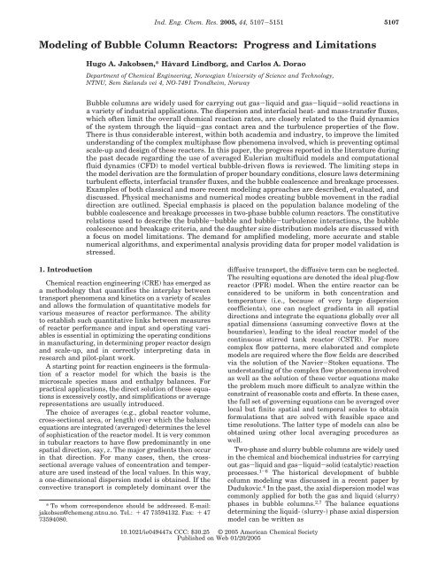
Ind. Eng. Chem. Res., Vol. 44, No. 14, 2005 5113Figure 4. Simulated steady-state results obtained with (s) and without (- --) the population balance at the axial level 2 m above thecolumn inlet. Points (‚) are experimental data. 76 v d s ) 8 cm/s.phases. 13 An alternative, often used when commercialCFD codes are used because of limited access to thesolver routines, is to solve the full two-fluid model inthe common way using the dispersed-phase continuityequation together with the two momentum equationsand the liquid-phase continuity. Within the IPSA-likecalculation loop, the N - 1 population balance equationsare solved in another step considering additional transportequations for scalar variables. Unfortunately, usingthis approach, it can be difficult to ensure mass conservationfor the dispersed phase, and/or negativeconcentrations can be predicted for the last class. Fromthe solution of the size distribution of the dispersedphase, the Sauter mean diameter is calculated. Thisdiameter is then used to compute the contact area, sothat the two-way interaction between the flow and thebubble size distribution is established. When dilutedispersions are considered, the interfacial momentumtransferfluxes due to particle collisions, coalescence,and breakage phenomena are normally neglected. Politanoet al. 62 are probably the only ones to have consideredthe interfacial momentum-transfer fluxes betweenthe bubble groups induced by bubble coalescence andbreakage, but still, they did not include the bubblecollisions resulting in rebound.Several recent studies indicate that algebraic slipmodels are sufficient for modeling the flow pattern inbubble columns, 13-15 as only the pressure and steadydragforces dominate the axial component of the gasmomentum balance. Therefore, the population balancemodel can be merged with an algebraic slip model toreduce the computational cost required for preliminaryanalysis. 66 Furthermore, by adopting this concept, therestriction used in the two-fluid model of assuming thatall of the particles have the same velocity can beavoided. This means that only one set of momentum andcontinuity equations for the mixture is solved, togetherwith the N population balance equations for the dispersedphases. The individual phase and bubble-classvelocities are calculated from the mixture velocitiesusing algebraic relations.Even simpler approaches are used in solving a singletransport equation for one moment of the populationbalance only, determining a locally varying mean particlesize or the interfacial area density. 36,67-69Luo 70 initiated the population balance investigationswithin our group. The main contribution was a closuremodel for binary breakage of fluid particles in fullydeveloped turbulence flows based on isotropic turbulenceand probability theories. 71 The authors also claimedthat this model contains no adjustable parameters,although a better phrase might be “no additionaladjustable parameters”, as both the isotropic turbulenceand probability theories involved contain adjustableparameters and distribution functions.Hagesaether et al. 72-75 continued the populationbalance model development within the framework of anidealized plug-flow model, whereas Bertola et al. 66combined the extended population balance module witha 2D algebraic slip mixture model for the flow pattern.Bertola et al. 66 studied the effect of the bubble sizedistribution on the flow fields in bubble columns. Theyused an extended k-ɛ model to describe the turbulenceof the mixture flow. Two sets of simulations wereperformed, i.e., both with and without the populationbalance. Four different superficial gas velocities, i.e., 2,4, 6, and 8 cm/s were used, and the superficial liquidvelocity was set to 1 cm/s in all cases. The populationbalance contained six prescribed bubble classes withdiameters set to d 1 ) 0.0038 m, d 2 ) 0.0048 m, d 3 )0.0060 m, d 4 ) 0.0076 m, d 5 ) 0.0095 m, and d 6 )0.0120 m.Figures 4 and 5 show simulated and experimentalresults for the superficial gas velocity v sg ) 8 cm/s.Figure 4 shows the axial and radial liquid velocity

5114 Ind. Eng. Chem. Res., Vol. 44, No. 14, 2005Figure 5. Calculated steady-state bubble number density at the axial level 2 m above the column inlet. Points (‚) are experimentaldata. 76 v d s ) 8 cm/s.components, the axial gas velocity component, and thegas fraction 2.0 m above the column inlet. Figure 5shows the number density in each class 2.0 m above theinlet.The results from the two simulations (i.e., with andwithout the population balance) are nearly identical. Inboth cases, the simulated results are in fair agreementwith the experimental data, but in the center of thereactor, the deviations between the simulated andexperimental velocity and void fraction profiles arerather large. The number density 2.0 m above the inletis shown in Figure 5. In general, it was found that theinitial bubble size was not stable and was furtherdetermined by break-up and coalescence mechanisms.The simulation provides results in fair agreement withthe experimental data for classes 3-6, for which thebubble number densities are of the same order ofmagnitude as the experimental data. In bubble classes1 and 2, the experimental bubble number densities areconsiderably underestimated in the simulations.However, in other cases, the model predictions deviatemuch more from each other and were in poor agreementthe experimental data on measurable quantities suchas phase velocities, gas volume fractions, and bubblesize distributions. An obvious reason for this discrepancyis that the breakage and coalescence kernels relyon ad hoc empiricism determining the particle-particleand particle-turbulence interaction phenomena.The existing parametrizations developed for turbulentflows are high-order functions of the local turbulentenergy dissipation rate that is often determined by thek-ɛ turbulence model. This approach is not accurateenough, 32,33,77 as this model variable (i.e., ɛ) merelyrepresents a closure for the turbulence integral lengthscale with model parameters fitted to experimental datafor idealized single-phase flows. The population balancekernels are also difficult to validate on the mesoscalelevel, as the physical mechanisms involved (e.g., consideringeddies and eddy-particle interactions) arevague and not clearly defined. If possible, the coalescenceand breakage closures should be reparametrizedin terms of measurable quantities. Well-planed experimentalanalysis of the mesoscale phenomena are thenrequired to provide data for proper model validation.Initial and Boundary Conditions. Initial andboundary conditions are also very important parts ofany model formulation. However, there is still verylimited knowledge regarding the formulation of properboundary conditions even for simple bubble columns. 11,12Inlet boundary conditions for the local gas volumefraction, bubble size distribution, and local gas velocitycomponents are difficult to determine, although anumber of more or less well founded suggestions havebeen reported in the literature. 43,66,78 The complex flowsin this section have been studied experimentally inseveral papers, 61,79,80 and there is clearly a need forimprovements as Harteveld et al. 61 found significantdiscrepancies between their experimental observationsand the present model predictions regarding the onsetof the significant flow instabilities. Harteveld et al. 61claimed that uniform aeration gives only a very smallentrance region and no large-scale circulation or coherentstructures. This visual observation clearly contradictsmost of the model predictions cited above.The specification of proper outlet boundary conditionsis also a problem for these flows, as the recirculatingmotion of the liquid phase continues as long as gasbubbles are present at sufficiently high fluxes. Consistentformulations of such boundaries have not yet beenreported. 81 This limitation restricts the use of explicitdiscretization schemes to situations with low gas fractionsor cases where the local recirculating flux containsvery little gas.For implicit solution methods, approximate and rathercrude outlet conditions are used for the flow variables.The boundary is usually idealized considering the liquid

Ind. Eng. Chem. Res., Vol. 44, No. 14, 2005 5115phase in batch mode only. 78 Following the experimentallaboratory practice of keeping the height of the gasliquiddispersion lower than the actual column height,the top surface of the column can be modeled as anoutlet for both the gas and liquid phases. It is anticipatedthat the solution of the model equations willdetermine the actual height of the gas-liquid dispersionand only gas will exit from the column outlet. Inadopting this approach, one has to ensure that themodeling closures are well posed and that the discretizationscheme applied to the governing equations aswell as the iterative solver used is capable of handlingthe steep gradients in the volume fraction and densityprofiles (discontinuities) that occur when the continuousphase change from being liquid below the gas-liquidinterface to gas above it. Because of the large densitydifference between these phases, such an attempt veryoften leads to nonphysical pressure and velocity valuesclose to the interface and encounters severe convergencedifficulties. To enhance the convergence behavior in theinterface region, empirically adjusted smooth profilesof the continuous-phase density profile and/or the voidfraction profile might help to maintain a fairly stablesolution. 82 For incompressible flows, this numericalapproach could enforce mass conservation, whereas forreactive and other density-varying systems, mass conservationcan be a severe problem so this boundarytreatment should be avoided.As numerical instabilities and inaccurate mass conservationare frequently encountered in solving problemscontaining sharp interfaces within the calculationdomain, the solution domain is often restricted to theheight of the gas-liquid dispersion. In this case, thelocal liquid velocity components normal to the outletplane are fixed at zero, as there is no net flux throughthe column outlet cross section. The top surface of thesolution domain is assumed to coincide with the freesurface of the dispersion, which might or might not beassumed flat. This assumption is rather crude, as anexact value of the gas-liquid dispersion height is notknown a priori. To induce apparently physical flowcharacteristics at the outlet, approximate boundariesare required for the other flow variables. The tangentialshear stress and the normal fluxes of all scalar variablesare set to zero at the free surface. The gas bubbles arefree to escape from the top surface. In commercial codes,this implementation might not be possible, and furtherapproximations have been proposed. In some cases, thetop surface of the dispersion is defined as an “inlet”where the normal liquid velocity is set to zero and thenormal gas velocity is set to an approximate terminalrise velocity. In other cases, the top surface of thedispersion is modeled as a “no shear wall”. This boundarysets both the gas and liquid velocities to zero. Torepresent escaping gas bubbles, an artificial gas sinkis defined for all of the grid cells attached to the topsurface. A similar approach was used by Lehr et al. 32The free surface assumed to be located at the top of thecolumn was replaced by an apparent semipermeablewall. In this way, the gas could leave the system,whereas the liquid surface acted as a frictionless wallfor the liquid. The liquid was considered to leave thesystem through an outflow at the periphery of thecolumn.Bove et al. 43 specified an outlet pressure boundaryinstead and determined the axial liquid velocity componentsin accordance with a global mass balance. Thisapproach is strictly valid only when the variations inliquid density due to interfacial mass transfer or temperaturechanges are negligible, as the local changesare not known a priori.Furthermore, in many industrial systems, the liquidphase is not operated in batch mode; rather, a continuousflow of the liquid phase has to be allowed. However,because of numerical problems, most reports on bubblecolumn modeling introduce the simplifying assumptionthat the continuous phase is operated in batch mode.Further work is needed on the continuous-mode boundaryconditions.The assumption of cylindrical axisymmetry in thecomputations prevents lateral motion of the dispersedgas phase and leads to an unrealistic radial phasedistribution that has also been reported by otherauthors. 35 Krishna and van Baten 35 obtained betteragreement with experiments when a 3D model wasapplied. However, experience shows that it is verydifficult to obtain reasonable time-averaged radial voidprofiles even in 3D simulations, even though the predictedradial velocity profiles seem reasonable.At the wall boundary, both the 2D and 3D turbulentviscosity-basedmodels rely on the assumption that thesingle-phase logarithmic law of the wall is still valid forbubble-driven upward flows in bubble columns. Troshkoand Hassan 83,84 claimed that this assumption is reasonablefor dilute and downward bubbly flows, but notrecommended for upward bubble-driven flows as foundin bubble columns. A corresponding two-phase logarithmicwall law was derived with the intention that itwould be in better agreement with experimental dataon homogeneous bubbly flows.Numerical Schemes and Algorithms. In terms ofprogress on the numerical side, several novel schemesand algorithms for solving the fluid dynamic part of themodel have been published (the solution methods intendedfor the population balance equation will bediscussed later). This work has concentrated on severalitems. Most important, as mentioned earlier, one avoidsusing the very diffusive first-order upwind schemeswhile discretizing the convective terms in the multifluidtransport equations. Instead, higher-order schemes, e.g.,second- or third-order TVD (total variation diminishing)schemes, which are much more accurate, have beenimplemented in the codes. 8,14,25,26,57 The numericaltruncation errors induced by the discretization schemeadopted for the convective terms can severely alter thenumerical solution, and this can destroy the physicsreflected by the model equations. It is also well-knownthat the strong coupling between the phasic equationsprevents efficient and robust convergence for the implicititeration process. 85 Exchanging the well-knownpartial elimination algorithm (PEA) of Spalding 86,87 andreducing the interaction between the phasic velocitiesin the drag terms of the momentum equations with acoupled solver 46,88-93 that simultaneously iterates on onevelocity component of all phases seems to improve thenumerical stability and the overall convergence rate. 94In addition, the discretization schemes together with thesolution algorithms lead to large sparse linear systemsof algebraic equations that need to be solved. Previously,the TDMA algorithm was applied to multidimensionalproblems to determine a linewise Gauss-Seidel approach.During the past decade, there have been developmentsin full-field solvers along the lines of Krylovsubspace methods and in the field of multigrid

5116 Ind. Eng. Chem. Res., Vol. 44, No. 14, 2005schemes. 90,91,94-96 These methods make effective use ofsparsity and are efficient methods for the solution oflarge linear systems. 96 Furthermore, the original interphase-slipalgorithm (IPSA) of Spalding 86 was developedto introduce an implicit coupling between pressure andvolume fractions. The algorithm contains an attempt toapproximate the simultaneous change of volume fractionsand velocity with pressure. However, most versionsof the IPSA algorithm were merely extensions ofthe single-phase SIMPLE approach; thus, the pressurewas computed by assuming that all of the velocitycomponents, but not the volume fraction variable,depend on pressure changes. The pressure-volumefraction relationship was not considered in a satisfactoryimplicit manner. Therefore, the extension of the singlephasepressure-velocity coupling to multifluid modelsled to low convergence rates and pure robustness of theiterating procedure. 20 Lately, numerical methods originallyintended for multiphase models, rather thanbeing extended single-phase approaches, have beeninvestigated. 46,89,91-93 A fully implicit coupling of thephasic continuity and compatibility equations within theframework of pressure-volume fraction-velocity correctionschemes seems to have potential if the resultingset of algebraic equations can be solved by an efficientand robust parallel solver. 93 However, so far, severestability problems have been identified within theiterative solution process. The numerical properties ofthe resulting set of algebraic equations are not optimizedfor robust solutions. In summary, significantimprovements of the numerics have been obtainedduring the past decade, but the present algorithms arestill far from being sufficiently robust and efficient.Further work on the numerical solution methods in theframework of FVMs should proceed along the pathssketched above. Very few attempts exploring the capabilitiesof alternative methods such as FEMs 97 and fullyspectral methods have been reported.Chemical Reaction Engineering. As a consequenceof the large number of modeling limitationsdiscussed above, caution concerning the predictivepower of the multifluid model applied to bubbly flowsis certainly justified. However, even though there areobviously many open questions and shortcomings relatedto the fluid dynamic modeling of bubble columns,preliminary attempts have been performed in predictingchemical reactive systems. For example, the early CFDmodels that were developed in our group to describeglobal steady flow pattern were tested aiming at predictingchemical conversion of a reactive system operatedin a bubble column. 20,98 The system investigatedwas CO 2 absorption in a methyldiethanolamine (MDEA)solution. The starting point for the numerical investigationwas a steady two-fluid flow model tuned to the air/water system. This air/water model was then appliedto the reactive system without retuning of any modelparameters but updating the physical properties inaccordance with the reactive system. It was found that,with this model, the global flow pattern, the interfacialmass-transfer fluxes, and the conversion were all stilldifficult to predict because of the limited accuracyreflected by the interfacial coupling models and especiallythe relations used for the contact area (and theprojected area). Several semiempirical models for thelocally varying mean bubble size and contact areas havebeen suggested 20,99 with limited success. The accuracyof the experimental data used for model validation wasalso questioned.According to Dudukovic et al., 5 still no fundamentalmodels for the interfacial heat- and mass-transfer fluxeshave been coupled successfully to the flow models, andreliable reactor performance predictions based on thesemodels are not imminent. The mechanisms of coalescenceand breakage are far from being sufficientlyunderstood yet.The physicochemical hydrodynamics determining thebubble coalescence and breakage phenomena cannot becaptured by any continuum model formulation. Therefore,the fluid dynamic models described above do notsignificantly improve on the prediction of the interfacialtransfer fluxes and thus the chemical conversion, as thepertinent physics on bubble, interface, and molecularscales still have to be considered using empirical parametrizations.A multiscale reactor model with aninherent two-way coupling between mechanisms onscales ranging from discrete molecular ones (moleculardynamics) to continuum macroscale reactor scales shouldbe elucidated. 100The weakest link in modeling reactive systems withinbubble columns is thus still the fluid dynamic part,considering multiphase turbulence modeling, interfacialclosures, and especially the impact and descriptions ofbubble size and shape distributions. For reactive systems,the estimates of the contact areas and thus theinterfacial mass-transfer rates are likely to contain largeuncertainties. The preliminary simulations performedto date clearly indicate that future work should alsoconsider the possibility of developing more efficient andstable numerical models for the integrated multiphase/population balance models. Bertola et al. 66 found thatthe CPU demand was increased by about 15% for everybubble class added to a simulation.Outline of the Paper. In the following sections, afairly rigorous modeling framework is outlined with afocus on population balance modeling. Emphasis isplaced on the closures for the coalescence and breakageterms. Bottlenecks that need further considerations areidentified. The numerical methods considered goodcandidates in solving the population balance model forbubbly flows are the moment, volume (i.e., the class andmultigroup), and spectral methods. The optimal choiceof numerical solution methods is discussed. Finally,concluding remarks are given.2. Modeling FrameworkAverage multifluid models with an integrated populationbalance module have been found to represent atradeoff between accuracy and computational efforts forpractical applications. If bubbles of different mass haveto be considered, separate continuity and momentumbalances are required for each bubble size and for thecontinuous liquid phase in a rigorous model formulation.The multifluid model equations are listed in thefollowing sections, together with the interfacial closuresthat are adopted in most gas-liquid (two-fluid) analyses.Multifluid Formulation. The multifluid model representsa direct extension of the well-known two-fluidmodel and is described in detail in Carrica et al., 13Pfleger et al., 30 Pfleger et al., 39 Tomiyama and Shimada,54 and Fan et al. 101 The governing set of equationsconsists of the continuity and momentum equations for

Ind. Eng. Chem. Res., Vol. 44, No. 14, 2005 5117N + 1 phases; one phase corresponds to the liquid phase,and the remaining N phases are gas bubble phases.The fundamental form of the multifluid continuityequation for phase k readswhere F k is the density and R k is the volume fraction ofphase k. The first term on the left-hand side denotesthe transient change of mass within a control volume,the second term denotes the convective flux of massthrough the surfaces of the control volume, and the termon the right-hand side describes the net mass-transferflux to phase k from all other phases l.The phasic volume fractions also satisfy the compatibilityconditionIn a consistent manner, the momentum balance forphase k yields∂∂∂t (R k F k ) + ∇‚(R k F k v k ) ) ∑Γ k,l (3)l)1The terms on the left-hand side of eq 5 denote the inertiaforce, whereas the terms on the right-hand side denoteall of the additional forces acting on phase k. These arethe pressure force, the deviating normal and shearstresses, the gravitational force, and the interfacialmomentum-transfer terms accounting for all momentumtransferfluxes between phase k and the other N phases.When sufficiently dilute dispersions are considered,only particle-fluid interactions are significant, and thetwo-fluid closures can be adopted. For the gas bubblephases (d), the interaction with the continuous liquidphase (c) and the wall (w) through the last term on theright-hand side of eq 5 is expressed asi.e., the sum of steady-drag, added-mass, lift, turbulentdiffusion, and wall forces, respectively. All of the forceterms are multiplied by the liquid fraction because ofthe reduced liquid volume available at considerable gasloadings.The net interfacial momentum-transfer term for theliquid phase (i.e., excluding the wall forces) can bewritten asThe drag force is given byNN+1∑ R k ) 1 (4)k)1∂t (R k F k v k ) + ∇‚(R k F k v k v k ) )-R k ∇p - ∇‚(R k σj k ) +NR k F k g +∑M k,l (5)l)1N+1∑ M d,l ≈ M d,c + M d,w )R c F d )R c F D,d +R c F V,d +l)1R c F L,d +R c F TD,d +R c F d,w (6)N∑d)1M c,d )-∑M d,c (7)d)1F D,d )-F D,d (v d - v c ) )- 34d s,dR d F c C D,d |v d - v c |(v d -Nv c ) (8)The drag coefficient can be estimated using the relationsuggested by Tomiyama et al. 102C D,d ) max{ min [ ARe B,d(1 +0.15Re B,d 0.687 ),For pure systems, the parameter A ) 16, whereas forcontaminated systems A ) 24. The Eötvös number, E 0,d ,is given asand Re B,d is the particle Reynolds number3ARe B,d] , 3E 0,d8(E 0,d + 4)} (9)E 0,d ) g z |F c -F d |d 2s,d(10)σ IRe B,d ) F c d s,d |v d - v c |µ c(11)The acceleration of the liquid in the wake of the bubblecan be taken into account through the added-mass forcegiven by Ishii and Mishima 103F V,d )-R d F c C V,d( Dv dDt - Dv cDt) (12)where C V,d ) 0.5 is derived for potential flow.The lift force on the dispersed phase due to shear inthe liquid phase is expressed as 104F L,d )-R d F c C L,d (v d - v c ) × (∇ ×v c ) (13)where C L,d ) 0.5 is derived for potential flow.The dispersion of bubbles in turbulent liquid flow canbe modeled as suggested by Carrica et al. 13F TD,d )-ν c,tR d Sc t,dF D,d ∇R d (14)where the Schmidt number is defined as Sc t,d ) ν c,t /ν d,t .An additional lift force that pushes the dispersedphase away from the wall was suggested by Antal etal. 105 to be given byF W,d ) max(0, C w1 + C w2d s,dy)R d F c|v d - v c | 2d s,dn w (15)where C w1 )-0.1 and C w1 ) 0.35. This force, eq 15,represents an extension of the original model of Antalet al. 105 A defect in the original model, namely, that abubble located far from the wall is attracted to the wall,has been removed. 63Turbulence Closures. It is expected that futuremultifluid models will adopt VLES turbulence closures.40 However, as noted in the Introduction, so far,the standard (single-phase) k-ɛ model is usually adoptedas the basis for describing liquid-phase turbulence inEulerian multiphase simulations. The structure of theturbulence model equations thus corresponds to thewell-known generalized scalar transport equation formultiphase flow. 39 A few extensions of the standard k-ɛmodel have also been used, accounting for bubbleinducedturbulence.The turbulence models adopted in the sample simulationspresented in this paper represent three versions

Ind. Eng. Chem. Res., Vol. 44, No. 14, 2005 5119- 1 F dn∫∇‚(R d / F d n v d /// )dv - 1 F cn∫∇‚(R c / F c n v c /// )dv)- ∆tF dn∫ V∇‚(R d / ∇φ n+1 )dv - ∆tF cn∫ V∇‚(R c / ∇φ n+1 )dv(26)5. The void fractions are updated by solving thecontinuity equation for the dispersed phase using thenewest estimate of the R k and v k variables∫ V( R n+1 d F n d -R n nd F d∆t) dv )-∫ V∇‚(R / d F n d v n+1 d )dv (27)For variable-density flows, a suitable equation of state(EOS) is used to calculate the variations in the densities.The fractional-step concept applied consists of successiveapplications of the predefined operators determiningparts of the transport equation. The convectiveand diffusive terms are further split into their componentsin the various coordinate directions. The timetruncationerror in the splitting scheme is of first order.The convective terms are solved using a second-orderTVD scheme in space and a first-order explicit Eulerscheme in time. The TVD scheme applied was constructedby combining the central difference scheme andthe classical upwind scheme by adopting the “smoothnessmonitor” of van Leer 108 and the monotonic centeredlimiter. 109 In the turbulence model, the diffusive termswere discretized with a second-order central differencescheme in space and a first-order semiimplicit Eulerscheme in time.4. Sample Results and DiscussionIn this section, the capabilities and limitations of 2Daxisymmetric two-fluid models for simulating cylindricalbubble column reactor flows are discussed. Modellimitations are explained, and sample results are givento illustrate the properties of the interfacial, turbulence,and wall interaction closures in use today. The aim isto evaluate whether a 2D model can be sufficient inproviding reasonable predictions when descriptions ofvariable bubble size distributions, chemical reactivesystems, continuous flow of the liquid phase, compressibleeffects, etc., are to be included in our fluid dynamicanalysis.In this work, simulations were performed with threedifferent turbulence closures for the liquid phase. Astandard k-ɛ model was used to examine the effect ofshear-induced turbulence (case a). In the first alternative,case b, both shear- and bubble-induced turbulenceare taken into account by linearly superposing theturbulent viscosities obtained from the k-ɛ model andthe model of Sato and Sekoguchi. 55 A third approach,case c, is similar to case b in that both shear- andbubble-induced turbulence contributions are considered.However, in this model formulation, case c, the bubbleinducedturbulence contribution is included through anextra source term in the turbulence model equations. 8As mentioned earlier, it has been shown by Svendsenet al., 17 among others, that the time-averaged experimentaldata on the flow pattern in cylindrical bubblecolumns apparently becomes close to axisymmetric.Therefore, it was anticipated that steady-state 2Daxisymmetric simulations could capture the pertinenttime-averaged flow pattern in these columns and thata time-averaged flow description was sufficient for theanalysis of interest for chemical reaction engineers.Because 2D computations are much faster to perform,it is also important to learn as much as possible fromsuch simulations before one performs dynamic 3Dcomputations that actually might not provide anyfurther information from a chemical engineering pointof view. Therefore, in line with the early CFD analysesof bubble column flows, in this work, we are merelyinterested in the time-averaged behavior of the flowsystem, comparing the model results with time-averagedexperimental data. As we proceed in discussingour results, we intend to reveal the pertinent reasonswhy this type of bubble column simulation has beenperformed for more than two decades with a ratherlimited degree of success.First, the lack of proper boundary conditions, asdiscussed in the Introduction, is further elucidated. Atthe column outlet, numerical problems arise for highersuperficial gas velocities, because of the intense recirculatingflow pattern produced by the free surfaceboundary that redistributes the liquid flow. Furthernumerical problems are observed for the case of operatingthe bubble column in a continuous liquid mode.The assumption of cylindrical axisymmetry in thecomputations prevents lateral motion of the dispersedgas phase and leads to an unrealistic radial phasedistribution wherein the maximum void is away fromthe centerline (Figures 6 and 7), as also reported byother authors. 35 Krishna and van Baten 35 obtainedbetter agreement with experiments by applying a 3Dmodel. Even though the time-dependent terms in our2D model were retained merely to ease the numericalsolution of the 2D pseudo-steady-state problem, so thatthe resulting transients predicted by our 2D model areconsidered numerical modes, it is interesting to notethat the flow development during the first 3-5 softhesimulations determines whether the fully developedsteady-state flow pattern will result in wall, intermediate,or center void peaking (apparently multiple steadystates). If the gas phase moves toward the wall or thecenter, there are no 3D secondary flows available toallow for any redistribution of the phases. Comparingour 2D axisymmetric model results at steady state withexperimental data on the axial velocities and voidfraction profiles at the axial level 0.3 m above the inlet,as in Figures 7 and 8, it can be observed that themagnitude of the simulated liquid axial velocity componentis overestimated at the centerline in cases a andc, whereas the higher effective viscosity level in case byields an estimation of the liquid axial velocity closerto the experimental results. The simulated axial velocitiesin the two phases are more tightly coupled than inthe experiment, resulting in overestimation of the axialgas velocity component at the centerline and underestimationtoward the wall. The corresponding void profileis in fair agreement with experiment, but with anunphysical local minimum at the center that has alsobeen observed by other investigators. The cross-sectionalaveragedvoid, however, is overestimated by about 25-35%, so the corresponding cross-sectional averaged gasvelocity is underestimated. This is an indication that3D effects are important at least in the inlet section.There is only one way to improve on this axisymmetricmodel limitation: a full 3D model is needed. However,studies reported in the literature show that it is verydifficult to obtain reasonable time-averaged radial voidprofiles even in 3D simulations, even though the pre-

5120 Ind. Eng. Chem. Res., Vol. 44, No. 14, 2005Figure 6. Axial liquid velocity, axial gas velocity, gas voidage, and viscosity profiles as a function of column radius at z ) 2.0 m after 80s (steady-state) using only drag and added mass as interfacial forces: ×, experimental data; 76 s, case a; ‚‚‚, case b; - - -, case c. Gridresolution, 20 × 72; time resolution, 2 × 10 -4 s.Figure 7. Axial liquid velocity, axial gas velocity, gas voidage, and viscosity profiles as a function of column radius at z ) 0.3 m after 80s (steady-state) using only drag and added mass as interfacial forces: ×, experimental data; 76 s, case a; ‚‚‚, case b; - - -, case c. Gridresolution, 20 × 72; time resolution, 2 × 10 -4 s.dicted radial velocity profiles seem reasonable. Alternatively,or rather in addition, the deviation betweenthe experimental data and the simulated results mightalso indicate that the inlet boundary conditions, phasedistribution, and interfacial coupling are inaccurate andnot in agreement with the real system, as will bediscussed later.The present simulations indicate that the most importantmechanism for radial movement of the gas, asthe gas starts entering the bottom of the column, is theliquid wall friction (Figure 8). In our 2D pseudotransientsimulations, the wall friction creates a significantpressure gradient at the inlet that pushes thegas toward the center line. An effect of the axisymmetricboundary condition is that it reflects most of themomentum in the fluid streams. Thus, if the effectiveviscosity in the bulk is low, only a small amount of thekinetic energy of the liquid will dissipate into heat, andthe reflected fluxes of liquid and gas might havesignificant radial velocity components. In contrast, atthe wall, the kinetic energy seems to be dissipated to alarger extent because of the wall friction. The radial

Ind. Eng. Chem. Res., Vol. 44, No. 14, 2005 5121Figure 8. Gas and liquid velocity components and gas voidageprofiles as a function of column radius showing center peaking inthe bubble column after 4 s (left) and 8 0s (right). Grid resolution,20 × 72; time resolution, 2 × 10 -4 s.boundary conditions thus make the radial flow unphysicallysensitive to the turbulence level in the column. Ifthe resulting radial velocity away from the center is highenough, a large fraction of the fluids seems to reach thewall, and the buoyancy force will ensure that the gasflows upward along the wall. This inlet flow patternresults in wall peaking, as shown in Figure 9. Alternatively,if the resulting radial velocity away from thecenter become lower because of a higher effectiveviscosity in the fluid phase, only negligible fluid streamswill reach the wall. The liquid will then entrain the gasdownward along the wall as the liquid continuityenforces a circulation cell, and a void center peakingprofile occurs as shown in Figure 8. Apparently, similarnumerical modes can be produced in dynamic 3Dsimulations with insufficient interfacial and turbulenceclosures.The limited accuracy reflected by the inlet boundarycondition and the prediction of bubble size distributionphenomena is considered next. The specifications ofproper inlet conditions for the phase distribution, localvelocities, bubble size distributions, turbulence quantitiesare not trivial. The approach used here relies onthe possibility of estimating an average bubble size orbubble size distribution at the inlet zone and a netterminal velocity and neglects the effects of the localFigure 9. Gas and liquid velocity components and gas voidageprofiles as a function of column radius showing wall peaking inthe bubble column after 4 s (left) and 8 0s (right). Grid resolution,20 × 72; time resolution, 2 × 10 -4 s.bubble jets found at the locations of the holes in the gasdistributor. This approach thus induces a diffusive effectdistributing the momentum uniformly over the columncross section. A better approach could be to resolve theflow through the gas distributor, as an integrated partof the model.Bertola et al. 66 studied the effect of the bubble sizedistribution on the flow fields in bubble columns usinga 2D axisymmetric mixture model with an inherentpopulation balance. The initial bubble size was foundnot to be stable and was further determined by breakupand coalescence mechanisms that were to a largeextent influenced by the local turbulence level. Even forthe pure flow calculations, the common simplifyingassumption of a uniform phase distribution at the inletwas found questionable, as the breakage and coalescencekernels rely on ad hoc empiricism determining theparticle-particle and particle-turbulence interactionphenomena. For reactive systems, the estimates of thecontact areas and thus the interfacial mass-transfer rateat the inlet are likely to contain large uncertainties.Turbulence model limitations are difficult to avoideven for single-phase flows. To enable multiphasesimulations with the k-ɛ model, a few model adjustmentswere required to avoid divergence of the numer-

5122 Ind. Eng. Chem. Res., Vol. 44, No. 14, 2005ical algorithms. Accounting for shear-induced turbulenceonly, case a, a minimum turbulent energy level,k min ) 5 × 10 -3 m 2 /s 2 , was used in the first few secondsof the pseudo-dynamic simulation to ensure a sufficientlyhigh viscosity level at the inlet to avoid havingthe turbulence level die out before the gas entered intothe column. For the same reason, the contribution ofthe bubble-induced turbulence in case b was enforcedby a factor of 10 during the first 3softhesimulationuntil the k-ɛ-model started to produce turbulent energy.In the case of introducing the bubble-induced turbulencethrough a source term in the turbulence model, case c,the start-up of the simulation was performed in thesame way as for case a.Comparisons between the steady-state profiles ataxial levels z ) 2.0 m and z ) 0.3 m for cases a-c aregiven in Figures 6 and 7, respectively. For z ) 2.0 m,all of the models give reasonable velocities comparedto the experimental data. The turbulent viscosity of caseb is approximately 20% higher than that of case a, whichresults in lower velocities that are closer to the experimentaldata. The turbulent viscosity profile in case clies between the two other profiles. However, thevelocities in case c are about equal to the velocities incase b.For z ) 0.3 m, there are larger discrepancies betweenthe simulated results and the experimental data, asdiscussed earlier. The voidage profiles observed in theexperiment are lower than at z ) 2.0 m, whereas theprofiles from the simulations are approximately thesame. The discrepancy indicates that the physics at thebottom of the column is not sufficiently captured by the2D model.The interfacial coupling and wall forces are difficultto parametrize with sufficient accuracy. However, thesteady-drag force is found to be the most importantinterfacial force in the system, as expected from literatureobservations. Reasonable agreement with experimentaldata is achieved by using this interfacial forceonly. A variety of different formulations of this force,and especially of the drag coefficient, can be found inthe literature, valid for deformable and spherical particlesand extended for different flow regimes, swarmeffects, and pure and contaminated fluid systems. Kuruland Podowski 111 compared several expressions for thedrag coefficient in a boiling channel and showed thatthe different correlations for bubbly flows appeared tohave minor effects on the predicted void fraction profiles.The different drag coefficients applied by Deen et al., 40Krishna and van Baten, 35 and Tomiyama 53 deviate byless than 15% in our simulations, indicating the accuracyof this parameter.However, in several papers on bubble column modeling,14,34 drag coefficient correlations valid for nondeformablespheres, 112,113 which give rise to drag forcecoefficients being about one-fourth the values of theother coefficients mentioned above for high Reynoldsnumbers, were adopted. When these spherical particlecoefficient correlations were applied in our simulations,all of the profiles became flat. The gas is thus not ableto entrain the liquid to the center in the bottom of thecolumn to create circulation cells. The literature profiles,on the other hand, seem very similar to the experimentaldata. It is speculated that this deviation can beexplained by the different grid arrangements used inthe different codes. It is believed, however, that the zerovoid fraction occurring at the wall should be considereda net effect of the forces acting on the bubbles, thusprescribing the wall void fraction results in an overconstrainedset of equations, and should be avoided. 105Further examination of these issues is required to avoidany misinterpretations of the physical phenomenainvolved.Implementing the added-mass force has barely anyinfluence on the steady-state solution; this conclusionis in agreement with the observations reported by Deenet al., 40 among others. Deen et al. 40 explained thisnegligible effect by the fact that the simulations yield aquasi-stationary state in which there is only a littleacceleration. The bubble jets observed close to thedistributor plate are then not considered. However, theconvergence rate and thus the computational costs aresignificantly improved when this force is implemented.The net effect of the transverse lift force is to pushthe gas radially inward or outward in the columndepending on the sign of the lift coefficient. The force isinduced by a velocity gradient and can therefore onlyreinforce or smooth out gradients in the flow fields. Inour 2D simulations, this force alone cannot change acenter peak flow pattern to a wall peak pattern or viceversa. This observation is quite surprising, as the flowpattern produced by the early steady-state model ofJakobsen 20 was totally dominated by this force. Areasonable explanation could be that the simulationsby Jakobsen 20 were strongly influenced by numericaldiffusion, as the resolution in the axial direction waslimited.Effects similar to those of the lift force are observedwhen a turbulent dispersion force that is proportionalto the gradient of the gas voidage is implemented. Theonly effect seen is that it smoothes out sharp gradientsin the domain until the profiles become completely flat,as the models tested seemed to overestimate the diffusioneffect. This trend is probably related to the lowaccuracy reflected by the effective viscosity variabledetermined by the turbulence model. The modeling ofthis force should also be seen in connection with theinherent numerical diffusion caused by the numericalapproximation of the convective terms.The radial wall lift force proposed by Antal et al. 105requires a certain minimum resolution of the grid closeto the wall. The choice of model coefficients is crucialfor the development of the profiles as these parametersdetermine the magnitude of the force as well as theoperative distance from the wall. The magnitude of theforce is highest for larger bubbles, and it seems to bevery sensitive to the bubble size. However, in our 2Dmodel simulations, the force could not be used to alterthe flow development significantly except very close tothe wall. There was no mechanism available for transportingthe gas further toward the center.Lopez de Bertodano 44 correctly suggested that severalunresolved phenomena close to the wall influence thephase distribution. A net axial friction force acting onthe gas in the vicinity of the wall was derived. In thepresent work, the net effect of this force is to reducethe time scale for the flow development from the gasstarts entering the column. However, this force has asignificant effect on the solution when the drag coefficientfor nondeformable spheres is used, as it causescenter peaking, whereas the profiles become flat withoutthis force as mentioned above. This indicates that a noslipcondition specified for the gas phase as well as afixed zero void fraction on the wall, which is used

Ind. Eng. Chem. Res., Vol. 44, No. 14, 2005 5123as boundary conditions in some numerical codes,will give reasonable results even with this drag coefficient.Another limiting model simplification adopted in mostreports on bubble column modeling is the assumptionof a constant gas density. Simulating columns that areseveral meters high, adopting an ambient pressureboundary at the outlet, cannot be consistent with thissimplifying assumption, as density gradient effectsbecome important. Similar inconsistency problems arisewhen reactive systems are simulated, as the gas densityhas to be allowed to vary in accordance with thechemical process behavior. In addition, in our experience,interfacial mass-transfer fluxes and chemicalreactions often induce numerical stability problems andthe lack of proper convergence.Finally, multiphase flow simulations are numericallyunstable considering both 2D and 3D models becauseof the applications of low-accuracy discretizations, largedensity differences between the phases, ill-conditionedimplementations of interfacial closures in the limit ofzero void or zero liquid fractions, and large gradientsor discontinuities in the flow fields that can occur inthese flow systems. Therefore, further studies on theseissue are highly recommended.Preliminary results using our 2D model show thataccurate discretization schemes for the dispersed-phasecontinuity equation and for the convection terms withinthe fluid momentum equations are crucial for accuratepredictions of the flow development. Large discretizationerrors can change the flow development from center towall peaking or visa versa. Similar observations werereported by Oey et al. 14 regarding the simulation of 2Drectangular columns in 3D.The physical interpretation and relevance of dynamic2D analysis of bubble column flows have been mattersof debate for many years. Judging from the experimentalanalyses discussed in the Introduction, it is evidentthat bubble column flows should be considered dynamicand 3D in any rigorous fluid dynamic analysis. Turbulenceis a dynamic 3D phenomenon. However, directnumerical simulations (DNS) of these systems is stillnot feasible, so some kind of filtering or averaging isneeded. Dynamic 3D simulations by use of filteredVLES models are computationally intensive and performaccurately only when the cutoff turbulence lengthscale (eddy size) is placed at a spectral gap in theturbulence energy spectrum, thereby ensuring that theenergy flux between the resolved and subgrid scales isvery small. Accurate modeling of these fluxes itself isthus necessary only when the subgrid-scale fluxes getlarge in comparison with the resolved fluxes (as in mostVLES simulations 114 ). Unfortunately, in engineeringpractice, the cutoff length scale is often apparentlychosen arbitrarily as no energy gap is found in theenergy spectrum, requiring more sophisticated subgridclosures. This might be one of the reasons why mostdynamic 3D simulations of bubble column flows havebeen performed using Reynolds-averaged models. Amongthe Reynolds-averaged turbulence models available, thesimple k-ɛ model is adopted in almost all of theinvestigations reported in the literature. There is experimentalevidence, however, that the flow in bubblecolumns is highly anisotropic. 115 It is thus an openquestion whether a 3D simulation using a k-ɛ model(predicting isotropic turbulence) provides the necessary3D effects or whether perhaps Reynolds stress or VLESmodels are required to represents the dynamics of theseflows. However, because of the impact of phenomenathat cannot be resolved by continuum models, it is notexpected that even the phase distributions predicted bythe use of VLES models will always be physicallyrealistic.Furthermore, when unsteady turbulent flow simulationsusing Reynolds-averaged models are performed,providing physical interpretations of the model resultsis not trivial. Schlichting and Gersten 116 suggested thatthese flow variables could be interpreted as timeaveragequantities whereby the time interval used inthe averaging operator had been chosen large enoughto include all turbulent fluctuations but still smallenough to contain no effect from the transient, orperiodic, parts. This concept is based on the assumptionthat the transient process occurs very slowly or that thefrequency of the oscillation is very small and lies outsidethe turbulent spectrum. Telionis 117 discussed an extensionof the standard Reynolds averaging approach: atriple decomposition, where the instantaneous quantitiesare decomposed into three parts. Recall that, in thestandard Reynolds decomposition, we split the instantaneousquantities into a time-independent time average(mean) and a fluctuation, whereas in the tripledecomposition approach, the mean motion is also dependenton time. The mean is thus generally made upof a time-independent part and a time-dependent part.In other cases, the application of the standard Reynoldsaveraging concept has been further extended to simulationsof transients that are within the turbulent spectrum.To compare the simulated results obtained withthis type of model with experimental data that areaveraged over a long time period to give steady-statedata (representing the whole spectrum of turbulence),both the modeled and the resolved scales have to beconsidered in much the same manner as for VLES. 118For bubbly flows, this model interpretation inducesanother severe problem related to the bubble-inducedturbulence phenomena. For steady-state simulationsusing the standard Reynolds-averaged models, theturbulent kinetic energy variable, k, denotes a measureof the mean energy considering all time scales withinthe flow (i.e., for the whole turbulence energy spectrum).In a typical energy spectrum, most of the energy isaccumulated on the larger scales of turbulence and verylittle on the smaller scales. This k quantity is thussometimes used as a measure of the energy level on theintegral scales (i.e., the larger energy containing scalesof turbulence). Considering the energy spectrum interms of turbulence length scales, the energy-containingscales represented by the k-ɛ model are thus normallymuch larger than the bubble size. The inclusion ofturbulence production due to the bubbles’ relativemotion is therefore based on the assumption of aninverse cascade of turbulence. 8 For dynamic simulations,the k quantity can represent scales less than orat the same order of magnitude as the particle size. Inthe cases where the time averaging operator is chosenin such a way that the dispersed phase is resolved, nobubble-induced turbulence mechanisms should be includedin the turbulence model.In summary, one can certainly conclude that dynamicsimulations of bubble column flows are not a trivial task.Physical interpretations of the simulated 3D dynamicsshould be performed with caution when any kind ofturbulence model is adopted.

5124 Ind. Eng. Chem. Res., Vol. 44, No. 14, 2005Considering the much simpler approach used in oursimulations, it was found that the 2D steady-statebubble column model has very limited inherent capabilitiesof predicting bubble column flows with sufficientaccuracy. However, after tedious adjustments of modelparameters, boundary conditions, time and space resolutions,numerical implementations, and solution algorithms,it is often possible to reproduce known flowfields to a certain extent. The global liquid flow patternis usually captured fairly well, whereas the correspondinggas fields are more questionable and difficult toevaluate because of the lack of reliable experimentaldata. Unfortunately, the possibility of achieving acompletely erroneous steady-state flow pattern wherethe liquid flows up along the wall and down in the coreof the column seems ever-present. The almost definitiverejection of this reactor model formulation is related tothe fact that it is often difficult to reproduce the gasvolume fraction fields with sufficient accuracy. Thelatter limitation would severely affect the contact areas,the interfacial heat- and mass-transfer fluxes, and theprojected areas, as well as the interfacial momentumtransferfluxes, making reliable predictions of theperformance of chemical processes impossible.It is speculated that the more specific model limitationsthat have to be eliminated to enable reliable modelpredictions can be found among the topics outlined inthe following. On the physical side, the model has to bemade 3D and dynamic, proper initial and boundaryconditions have to be formulated, the high-frequencyturbulence mechanisms and lower-frequency coherentstructures have to be resolved (requiring sufficientlyaccurate turbulence closures), the fluid particleturbulenceinteraction mechanisms as well as interparticleinteractions are probably important, the descriptionof the interactions between the dispersedphase and the turbulent wall boundary layer structureshould be extended, the pertinent phase distributionmechanisms have to be identified and described withsufficient accuracy, bubble size and shape distributionshave to be considered (i.e., the microscopic bubblecoalescence and breakage processes have to be described),the interfacial momentum closures have to bedescribed with higher accuracy (especially the transverseforces), the free surface at the top of the columnmight have to be resolved, the mechanical and turbulenceenergy balances in the system have to be fulfilled(for validation of the interfacial transfer fluxes and theenergy dissipation rates), phasic density variationsshould be allowed, and the impact of heat- and masstransfermechanisms and chemical conversion mightneed to be investigated in further detail. On the numericalside, any algorithms, grid arrangements, unphysicalsource implementations (e.g., unphysical modelextensions implemented to avoid ill-conditioned implementationsof interfacial and turbulence closures in thelimit of zero void fractions), or discretization truncationerrors producing solutions merely determined by numericalmodes rather than physical mechanisms shouldbe removed (if possible). Finally, proper convergencecriteria should be formulated and fulfilled for every timestep in the simulation.In view of the comprehensive list of limitationsprovided above, it is concluded that a truly predictivemodel is not imminent. However, the more pressingimprovements required soon are those that will enablea sufficiently accurate description of the time-averagedphase distribution in the system. These improvementsshould also ensure that one would not achieve, on atime-averaged basis, downward flow of liquid in the coreof the column and upward flow of liquid close to the wallthat completely disagree with the available experimentalobservations. The authors believe that, in thiscontext, one of the most important model extensionsrequired is the inclusion of a proper description of thebubble size and shape distributions. Further work inour group continues to elucidate these issues along thelines described in the remaining sections of this paper.5. Population Balance FrameworkThe chemical engineering community began the firstefforts of association with the concepts of the populationbalance in the 1960s.Two fundamental modeling frameworks emerge forformulating the early population balances, in quite thesame way as the kinetic theory of gases and thecontinuum theory were proposed deriving the governingconservation equations in fluid mechanics (e.g., appendixesin Williams 119 ). A third less rigorous approachis also used in formulating the population balancedirectly on the volume-averaging scale considering theinternal coordinates (i.e., particle size), an analogue tomultiphase mixture models.Considering dispersed two-phase flows, a few researchgroups have thus preferred to describe the dispersedphase on the basis of a statistical Boltzmann-typeequation determining the temporal and spatial rates ofchange of a suitably defined distribution function.Performing “Maxwellian” averaging, integrating allterms over the whole velocity space to eliminate thevelocity dependence, one obtains the generic populationbalance equation. Reliable closures are required for theunknown terms resulting from the averaging process.However, this theory provides rational means of understandingthe one-way coupling between discrete particlephysics and the average continuum properties. Theprocedure sketched above has much in common with thegranular theory (i.e., that could be defined as the flowof powder in a vacuum) of solid particles. 120 However,the great majority of research groups within the chemicalengineering community adopted an approach basedon an extension of the classical continuum theoryinstead developing the population balance equation. Themain reason for this choice was probably that the basicconcept is familiar to most chemical engineers frombasic courses in fluid mechanics, whereas the principlesof kinetic theory might be less accessible from a pedagogicpoint of view. On the other hand, the continuumtheory gives only an average representation of thedispersed phase (i.e., on a macroscopic level relative tothe particle scale) and does not provide any informationon the unresolved mechanisms formulating the populationbalance closures. In most cases, the balance principleis applied by formulating the particle numberbalance on the integral form. Extended versions of theLeibnitz and Gauss theorems are then required totransfer the integral balances to the differential form.For turbulent flows, the governing microscopic continuumequations on the differential form are then time-(Reynolds-) averaged after being volume averaged toobtain trackable volume and time resolutions, givingrise to additional closure requirements. 121 The thirdgroup of population balances are thus formulated directlyon the averaging scales.The Leibnitz and Gauss

Ind. Eng. Chem. Res., Vol. 44, No. 14, 2005 5125theorems are used to cast all of the terms in theequation into a volume integral. The governing integralequation is thereafter converted to the differential form.In this formulation, the closures are purely empiricalparametrizations based on intuitive relationships ratherthan sound scientific principles.Even though the kinetic theory approach is consideredmore general, the basic balance formulation might needto be reformulated for every novel system consideredto ensure that the pertinent physics on the discreteparticle level is consistent with the problem in question.An optimized choice of distribution function definitionmight be necessary, and novel closures might be required,making the approach rather demanding theoretically.The population balance concept was first presentedby Hulburt and Katz. 122 Rather than adopting thestandard continuum mechanical framework, 123 the modelderivation was based on the alternative continuumapproach based on particle statistics familiar fromclassical statistical mechanics. The main problemsinvestigated stem from solid particle nucleation, growth,and agglomeration.Randolph 124 and Randolph and Larson, 125 on theother hand, formulated a generic population balancemodel based on the extended continuum mechanicalframework. Their main concerns were solid particlecrystallization, nucleation, growth, agglomeration/aggregation, and breakage.Ramkrishna 126,127 adopted the concepts of Randolphand Larson to explore biological populations. An outlineof the population balance model derivation from thecontinuum mechanics point of view was discussed.Similar approaches are also frequently used in thetheory of aerosols in which the gas is the continuousphase 121,128 and in chemical, mechanical, and nuclearengineering describing multiphase droplet flow dynamics;129,130 such an approach was also used for incompressiblebubbly two-phase flows by Guido Lavalle etal. 131Carrica et al. 13 developed the population balance fromkinetic theory using the particle mass as the internalvariable while investigating compressible bubbly twophaseflow around a surface ship, whereas most earlierwork on solid particle crystallization used particlevolume (or diameter). The two formulations are completelyequivalent in the case of incompressible gases.However, in flows where compressibility effects in thegas are important (as in the case of experimental bubblecolumns operated at atmospheric conditions), the useof mass as an internal variable was found to beadvantageous because it is conserved under pressurechanges. Lehr et al., 32 Millies and Mewes, 68 Lehr andMewes, 36 and Pilon et al. 132 sketched a possible alternativeformulation using particle volume (diameter) as theinternal coordinate. In their approach, several growthterms have to be considered to express the effects of gasexpansion due to changes in gas density in accordancewith a suitable EOS. The use of a mass density form ofthe population balance derived according to the kinetictheory approach (i.e., instead of the more commonnumber density) has also been discussed, having severaladvantages in reactor technology. 133,134In chemical engineering, Coulaloglou and Tavlarides135 were among the first to introduce the simplermacroscopic formulation, describing the interactionprocesses in agitated liquid-liquid dispersions. Driftingfrom the fundamental equations, the closures becamean integrated part of the discrete numerical discretizationscheme adopted (i.e., there is no clear split betweenthe numerical scheme and the closure laws).Lee et al. 136 and Prince and Blanch 77 adopted thebasic ideas of Coulaloglou and Tavlarides 135 to formulatethe population balance source terms directly on theaveraging scales to perform an analysis of bubblebreakage and coalescence in turbulent gas-liquid dispersions.The source term closures were completelyintegrated parts of the discrete numerical schemeadopted. The number densities of the bubbles were thusdefined as the number of bubbles per unit mixturevolume and not as a probability density in accordancewith the kinetic theory of gases.Luo and Svendsen 71 extended the work of Coulaloglouand Tavlarides, 135 Lee et al., 136 and Prince and Blanch, 77formulating the population balance directly on themacroscopic scales where the closure laws for the sourceterms were integrated parts of the discrete numericalscheme used to solve the model equations. The worksof Millies and Mewes, 68 Lehr and Mewes, 36 Lehr et al., 32Hagesaether et al., 73-75 and Wang et al. 137 all adoptedthe governing population balance of Luo and Svendsen.71The extension of these modeling concepts to bubbledrivengas-liquid flows is not as straightforward as onemight think from either a physical or a computationalpoint of view. Many physical or physicochemical mechanismsare still not understood or possibly even notdiscovered yet, and as the pertinent interfacial phenomenainvolved are expected to interfere at the molecularscale, tremendous computational efforts arerequired. Further challenges are foreseen consideringreactive systems in industrial chemical reactors, as thechanges in species compositions, heats of reaction, andsurface processes are strongly linked.However, preliminary attempts have already beenmade in the modeling of bubble coalescence and breakagein gas-liquid systems, adopting the populationbalance framework and mathematical modeling toolsproposed by the above-mentioned pioneers. Integratedmultiphase flow/population balance models have beenapplied to bubble column reactors and two-phase stirredvessels with limited success. 31,32,41,65,66,138,139 The simulationsreveal that these models are not able to predictnonequilibrium bubble size distributions sufficientlyaccurately as a function of space and time because ofthe very restricted predictive capabilities reflected bythe present population balance kernels for both bubblecoalescence and breakage.In the following subsections, two forms of the populationbalance are formulated in accordance with thecontinuum theory. First, a macroscopic balance isformulated directly on the averaging scales in terms ofnumber density functions. A corresponding set of sourceterm closures is presented as well. Second, a morefundamental microscopic population balance as well asfairly general expressions for the source terms areformulated in terms of number probability densities.This balance is then averaged using the popular timeafter-volumeaveraging procedure. The fairly generalform of the constitutive relations adopted for the bubblecoalescence and breakage phenomena are formulatedpurely on the basis of physical reasoning and intuitiveinterpretations of the mechanisms involved. Furtherlinks to the discrete particle-scale phenomena areusually expressed on the averaging scales by extrapo-

5126 Ind. Eng. Chem. Res., Vol. 44, No. 14, 2005lating relationships and concepts from the kinetic theoryof gases. However, the basic kinetic theory of gases doesnot provide any coupling between the particles and theambient fluid. In a more generalized framework, however,the kinetic theory concept allows for the introductionof external forces determining the interactionbetween the fluid and the dispersed particles. Theapproach described by Ramkrishna 127 is outlined.Macroscopic Population Balance Equation. Inthis subsection, the macroscopic population balanceformulation of Luo 70 is outlined. In the work of Luo, 70no growth terms were considered; the balance equationthus contained a transient term, a convection term, andfour source terms due to binary bubble coalescence andbreakage. The population equation was expressed as∂n i∂t + ∇‚(v i n i ) ) B B,i - D B,i + B C,i - D C,i ( 1sm 3)(28)where n i is the number density with units of 1/m 3 andv i is the mass-average velocity vector, v i ) (∑ N i)1 -n i v i,p F g V i )/(∑ Ni)1 n i F g V i ). [Note that, alternatively, theparticle number-average, v i,ni ) (∑ N i)1 n i v i,p )/(∑ N i)1 n i );size-average, v i,di ) (∑ N i)1 n i v i,p d i )/(∑ Ni)1 n i d i ); surface-average,v i,ai ) (∑ N i)1 n i v i,p a i )/(∑ Ni)1 n i a i ); or volume-average,v i,Vi ) (∑ N i)1 n i v i,p V i )/(∑ Ni)1 n i V i ) velocity vector could beused as well. 140 ] The source terms express the bubblenumber birth and death rates per unit dispersionvolume for bubbles of size d i at time t due to coalescenceand breakage. The source terms are assumed to befunctions of bubble size d i , bubble number n i , and timet.The birth of bubbles of size d i due to coalescence stemsfrom the coalescence between all bubbles of size smallerthan d i . Hence, the birth rate for bubbles of size d i , B C,i ,can be obtained by summing all coalescence events thatform a bubble of size d i . This givesB C,i )d i /2∑ Ω C (d j :d i - d j )d j )d min( 13) (29)smwhere d min is the minimum bubble size and depends onthe minimum eddy size in the system. The source termdefinition implies that bubbles of size d j coalesce withbubbles of size (d i - d j ) to form bubbles of size d i . Theupper limit of the sum stems from symmetry considerationsor avoidance of counting the coalescence betweenthe same pair of bubble sizes twice.Similarly, the death of bubbles of size d i due tocoalescence stems from coalescence between two bubblesin class d i or between one bubble in class d i and otherbubbles. Hence, the bubble death rate for bubbles of sized i , D C,i , can be calculated asd max -d iD C,i ) ∑ Ω C (d j :d i )d j )d min( 13) (30)smwhere d max is the maximum bubble size in the system.The upper limit indicates that the bubble size formedby coalescence must not exceed d max .The birth of bubbles of size d i due to breakage stemsfrom the breakage of all bubbles larger than d i . Thebreakage birth rate, B B,i , can be obtained by summingall breakage events that form bubbles of size d id maxB B,i ) ∑ Ω B (d j :d i )d j )d i( 13) (31)smThe death of bubbles of size d i due to breakage stemsfrom breakage of bubbles within this class; thusD B,i ) Ω B (d i )( 1sm 3) (32)The local gas volume fraction in any grid cell can becalculated as R g ) ∑ N i)1 n i (π/6)d 3 i .The macroscopic model formulation has numericalproperties similar to those of the discrete discretizationscheme (discussed later) and can be solved directlywithout further considerations.To ensure number and mass conservation, Hagesaetheret al. 73-75 extended this model by adopting anumerical procedure to redistribute the bubbles on pivotpoints in accordance with the discrete solution method.This modification of the solution strategy was introducedbecause of an inherent model limitation, i.e., thebreakage closure of Luo and Svendsen 71 was not necessarilyconservative, as will be explained later.Macroscopic Source Term Closures. In accordancewith the work of Coulaloglou and Tavlarides 135and Prince and Blanch, 77 Luo 70 assumed that allmacroscopic source terms determining the death andbirth rates could be defined as the product of a collisiondensity and a probability. Thus, modeling of bubblecoalescence means modeling of a bubble-bubble collisiondensity and a coalescence probability, whereasmodeling of bubble breakage means modeling of aneddy-bubble collision density and a breakage probability.Models for the collision densities were derived assumingthat the mechanisms of the bubble-bubble andeddy-bubble collisions are analogous to those of collisionsbetween molecules as in the kinetic theory ofgases. 135Models for the Binary Bubble Coalescence Rate,Ω C (d i :d j ). For coalescence between bubbles of class, d i ,and bubbles of class, d j , the coalescence rate is expressedasΩ C (d i :d j ) ) ω C (d i :d j ) p C (d i :d j )( 1sm 3) (33)Models for the Bubble-Bubble Collision Density,ω C (d i :d j ). Although not necessarily valid for bubblecolumns, the dispersions are considered sufficientlydilute that only binary collisions need to be considered.A collision of two bubbles can occur when the bubblesare brought together by the surrounding liquid flow orby body forces such as gravity. At least three sources ofrelative motion can be distinguished: motion inducedby turbulence in the continuous phase; motion inducedby mean velocity gradients; and motion induced bybuoyancy (or, more generally, body forces) arising fromdifferent bubble slip velocities, wake interactions, orhelical/zigzag trajectories. 140 However, most studies onbubble columns have been restricted to considering onlymodels for the contribution of turbulence to coalescence;the contributions from mean velocity gradients and bodyforces are generally neglected without proper validation.These collision mechanisms are generally both signifi-

Ind. Eng. Chem. Res., Vol. 44, No. 14, 2005 5127Figure 10. Sketch of a collision tube of an entering bubble movingthrough the tube with a velocity v p. The bubbles within the tubeare assumed to be “frozen” or stationary.cant, which greatly complicates the construction andvalidation of coalescence models.The parametrization of the collision densities wasobviously influenced by the more fundamental studieson formulating the source terms at the microscopic levelfollowed by some kind of averaging and a discretenumerical discretization scheme, as will be furtheroutlined in a later section. At this point, it is simplyobserved that the units of the volume-average coalescencefrequency correspond to the units of the effectiveswept volume rate in the kinetic theory of gases.Therefore, rather than the actual collision density, thevolume swept by a moving particle (i.e., bubble or eddy)multiplied by the particle density squared is used todefine the collision densities. 77,135,138To derive an expression for the effective swept volumerate, one usually considers a particle as it travels in astraight path from one collision to the next in amonodisperse dispersion, as sketched in Figure 10. Theparticle’s speed and direction of motion changes witheach collision. Further imagine that, at a given instant,all particles except for the one in question are frozen inposition and this particle moves with an average speed,v p . At the instant of collision, the center-to-centerdistance of the two particles is d. The collision crosssection of the target area of the particle is σ A ) 1 / 4 πd 2 .It should be noted that the collision cross-sectional areais defined in several ways. In one approach, inspiredby kinetic theory, the moving particle is approximatedas a point-like particle. Thus, the cross section of themoving particle is not considered in calculating theeffective cross-sectional area; hence, σ A ) 1 / 4 πd 2 .Inthecase of small particles, this approximation might besufficient. However, an improved estimate of the effectivecross-sectional area is achieved by taking intoaccount the size of the moving particle as well; thus σ A) πd 2 , as sketched in Figure 11. In time ∆t, the movingparticle sweeps out a cylindrical volume of length v p ∆tand cross section 1 / 4 πd 2 . Any particle whose center isin this cylinder will be struck by the moving particle.The number of collisions in the time ∆t is f 1 ( 1 / 4 πd 2 v p ∆t),where f 1 is assumed to be locally uniformly distributedin space. The effective swept volume rate h C (d) is givenbyh C (d) ) σ A v p ) 1 4 πd2 v p( m3s) (34)where σ A ) 1 / 4 πd 2 is the cross-sectional area of the socalled“collision tube”.Figure 11. Sketch of a collision tube of a bubble, defining thecollision diameter and the effective cross-sectional area.The collision density of a single particle is defined asthe number of collisions per unit time and length(diameter)ω f1(d) ) f 1 (d) h C (d) ) f 1 (d,t) 1 14 πd2 v p [(35)s (m)]This relation represents a very crude collision model fora dispersion containing only one type of particle.Sometimes, the collision density representing thenumber of collisions per unit mixture volume and perunit time and length (diameter) is a more convenientquantity. Multiplying the collision density of a singleparticle by the particle number density, one obtains themodified collision densityω f1 f 1(d) ) h C (d) f 1 f 1 ) 1 2 f 1 f 1114 πd2 v p[ m 3 s (m) (m)](36)The factor of 1 / 2 appears because h(d) represents twicethe number of collisions.In accordance with the pioneering work of Smoluchowski,141 similar considerations can be repeated fordispersions containing two types of particles havingdiameters d, d′ and particle densities f 1 , f′ 1 . The resultingcollision density is given byω C (d,d′) ) h C (d,d′) f 1 f′ 1 )πf 1 f′ 14( d + d′1vrel2 )2[ m 3 s (m) (m)] (37)where the collision frequency is calculated using themean collision diameter d ≡ (d + d′)/2, as sketched inFigure 12. Note that, in this case, the 1 / 2 factor is notincluded.Kolev 130 discussed the validity of these relations forfluid particle collisions considering the obvious discrepanciesresulting from the different nature of the fluidparticle collisions compared with the random molecularcollisions. The basic assumptions in kinetic theory thatthe molecules are hard spheres and that the collisionsare perfectly elastic and obey the classical conservationlaws do not hold for real fluid particles because theseparticles are deformable and elastic and can agglomerateor even coalesce after random collisions. The collisiondensity is thus not truly an independent functionof the coalescence probability.

5128 Ind. Eng. Chem. Res., Vol. 44, No. 14, 2005subrange of turbulence, then δv 2 (d) ) C(ɛd) 2/3 . A relationshipbetween the constant C and the Kolmogorovconstant C k (i.e., the parameter in the energy spectrumfunction for the inertial subrange) can be deduced fromthe power-law spectrum and the second-order structurefunction, C ) (27/55)Γ(1/3)C k . 144,145 Setting C k ) 1.5 inaccordance with experimental data yields C ≈ 2.0.Interpreting the second-order structure function (i.e.,because it is a two-point correlation function) as arelative particle velocity (i.e., actually a mean velocityobtained using one-point statistics seems more appropriate),the collision density suggested by Prince andBlanch 77 becomesFigure 12. Sketch of the mean collision diameter and the effectivecross-sectional area.As mentioned above, bubble-bubble collisions canoccur as a result of a variety of mechanisms. Prince andBlanch 77 modeled bubble coalescence in bubble columnsconsidering bubble collisions due to turbulence, buoyancy,and laminar shear through analysis of the coalescenceprobability (efficiency) of collisions. It wasassumed that the collisions from the various mechanismswere cumulative.The collision density resulting from turbulent motionwas expressed as a function of bubble size, concentration,and velocity in accordance with the work ofSmoluchowski 141ω T π(d,d′) ≈ f 1 f′ 14( d + d′ 22 )2 (vjt,d + vj 2 t,d′ ) 1/21m 3 s (m) (m)] (38)Estimates of the turbulent velocities have been obtainedusing certain relations developed in the classicaltheory on isotropic turbulence due to Kolmogorov. 142 Atthis point, the population balance closures seem tobecome rather vague, as the application of the classicalturbulence relations developed for fluid velocity fluctuationsor vortices to describe flows of discrete fluidparticles are not always in accordance with the basicturbulence theory restrictions. The theory of Kolmogorov142 states that, if the distance λ between two pointsin the flow field is much smaller than the turbulencemacroscale L but much larger than the Kolmogorovmicroscale λ d , then the second-order velocity structurefunction is a function of only the turbulent energydissipation rate ɛ and the magnitude of the length λ,δv 2 (λ) ) C(ɛλ) 2/3 . This two-point velocity structurefunction should not be confused with the normal componentof the Reynolds stresses, which is a one-pointvelocity correlation function.A summary of the theory involved is given by Pope 143(Chapter 6 and Appendix G). By definition, the secondordervelocity structure function is the covariance of thedifference in velocity between two points in physicalspace. Considering the second-order structure functiondefined by Kolmogorov 142 for the continuous fluid flowturbulence, it can be expressed at a separation equal tothe bubble diameter d as δv 2 (d) ) [v z (z+d)-v z (z+d)] 2 .If the magnitude of diameter d lies within the inertial[ω T πC (d i :d j ) ≈ n i n j4( d i + d j2) 2 (vj t,di + vj t,dj ) 1/2 ≈0.089πn i n j (d i + d j ) 2 ɛ 1/3 (d 2/3 i + d 2/3 j ) ( 1/2 1 ) (39)sm 3(Note that the collision density was originally expressedin accordance with the macroscopic population balance.70 If otherwise acceptable, it seems that the coalescenceclosures formulated directly within the macroscopicframework can be transformed and expressedin terms of probability densities and used within theaverage microscopic balance framework without furtherconsiderations if one adopts a discrete numerical discretizationscheme.)Note that the parameter value used by Luo 70 and Luoand Svendsen 71 is a factor of 4 larger than this, one asthey used a different definition of the effective crosssectionalarea.In this interpretation, two bubbles being dispersed ina large-scale fluid eddy (i.e., larger than the bubblescale, d) are assumed to be advected together with thefluid without approaching each other.However, the validity of the Kolmogorov hypothesisdescribing bubbly flows is not yet strictly verified. Forconvenience, the relationship for turbulent fluid velocityfluctuations has thus been interpreted and extrapolatedin many ways. There seems to be some confusion in theliterature regarding different interpretations of theKolmogorov velocity scale and the second-order structurefunction. 143 The second-order structure function,δv 2 (d), has thus (apparently erroneously) been used asan estimate for an imaginary absolute turbulent bubblevelocity in the inertial subrange of isotropic turbulence,in other cases considered a relative bubble velocity in aturbulent flows, 77 and as a third possibility been useda measure of intrabubble oscillations.The buoyancy collision density ω B C (d i :d j ) is expressedas (Prince and Blanch; 77 Williams and Loyalka, 128 p 164)ω B πC (d i :d j ) ≈ n i n j4( d i + d j2) 2 |vj r,di - vj r,dj | ( 1 )sm 3 (40)where vj r,di is the rise velocity of the particle. (Again, notethat the collision density was originally expressed inaccordance with the macroscopic population balanceformulation. 70 )The functional form of the collision rate due tolaminar shear is given by (Friedlander, 121 p 200; Williamsand Loyalka, 128 p 170)

)3( ω LS 4C (d i :d j ) ≈ n i n j3 (d i + d dv cjdR) ( 3) 1 (41)smwhere v c is the continuous-phase circulation velocity andR is the radial coordinate of the column. The term(dv c /dR) is the average shear rate. [Again, the collisiondensity was originally expressed in accordance with themacroscopic population balance formulation (e.g, Luo 70 ).]The net coalescence frequency of bubbles of diametersd i and d j was then calculated by superposing thedifferent bubble collisions mechanisms as a linear sumof contributions multiplied by a common efficiency (asimilar closure can be obtained for the average microscopicformulation if one adopts a discrete numericaldiscretization scheme, as will be described later) 77p C ∝ f(∆t coal /∆t col ) (44)The coalescence efficiency thus represents the fractionof particles that coalesce out of the total number ofparticles that have been colliding. The functional relationshipgiven by Coulaloglou and Tavlarides, 135 i.e.p C ≈ exp(-∆t coal /∆t col ) (45)is often used for the modeling of bubble coalescenceprobabilities for bubble column flows.Ω C (d i :d j ) ) [ω T C (d i :d j ) + ω B C (d i :d j ) +The duration of such interactions is limited, andcoalescence will occur only if the intervening film canω LS C (d i :d j )]p C (d i :d j )( 1drain to a sufficiently small thickness to rupture in thesm3)(42)time available.Coalescence is obviously possible if there is enoughHagesaether 146 adopted this approach when modeling contact time for completing the coalescencebubble column dispersions and found that, with thechoice of parameter values used in his analysis, the∆t col > ∆t coal (46)turbulent contribution dominated the collision rate forthe bubbles in the system. However, the most important Luo, 70 Luo and Svendsen, 71 and Hagesaether et al. 73-75model parameter as the turbulent energy dissipation adopted this approach.rate is difficult to compute, and only crude estimates The complexity of the film draining phenomenawere obtained. 32,70,77 In addition, Kolev 130 argued that involved is a severe problem and might be best illustratedby briefly discussing an early modeling at-the frequency of coalescence of a single bubble shouldrather be determined for individual efficienciestempt. Oolman and Blanch 147 derived an expression forthe coalescence times in stagnant fluids by examiningΩ C (d i :d j ) ) ω T C (d i :d j ) p T C (d i :d j ) + ω B C (d i :d j ) p B C (d i :d j ) + the time required for the liquid film between bubblesto thin from an initial thickness to a critical value whereω LS C (d i :d j ) p LS C (d i :d j ),( 13) sm (43)Kolev 130 further assumed that, for the coalescenceprocesses induced by buoyancy and nonuniform velocityfields, the forces leading to collisions inevitably acttoward coalescence for contracting particle free paths.Therefore, the probabilities must have the followingranges: 0 E p C T (d i :d j ) E 1 and p C B (d i :d j ) ) p C LS (d i :d j ) ≈ 1.However, no firm conclusions on the relative importanceof the various contributions have yet been drawn,as the turbulent particle velocity closures are at bestinaccurate.Models for the Probability of Coalescence, p C -(d i :d j ). The probability or efficiency of oscillatory bubblecoalescence, e.g., induced by turbulent fluctuations, isexpected to be determined by physical mechanisms onvarious scales. The coalescence process is assumed tooccur in three consecutive stages. First, bubbles collide,trapping a small amount of liquid between them underthe action of the continuous phase. Second, this liquidthen drains over a period of time from its initialthickness until the liquid film separating the bubblesreaches a critical thickness, under the action of the filmhydrodynamics. The hydrodynamics of the film dependson whether the film surface is mobile or immobile, andthe mobility, in turn, depends on whether the continuousphase is pure or a solution. Third, at this point, filmrupture occurs because of film instability, resulting ininstantaneous coalescence (i.e., usually not modeled infurther detail). The probability of coalescence is thusdefined as a function of the ratio of the time intervalwithin which the bubbles are touching each other, calledInd. Eng. Chem. Res., Vol. 44, No. 14, 2005 5129the collision time interval, ∆t col , and the time intervalrequired to push out the surrounding liquid and toovercome the strength of the capillary microlayer betweenthe two bubbles, called the coalescence timeinterval, ∆t coal130rupture occurs. The original model considers the flowrate of fluid from the liquid film by capillary pressure,augmented by the Hamaker contribution (reflecting themutual attraction of fluid molecules on opposite sidesof the liquid film) at very low film thicknesses, bubbledeformation, and the changes in the concentration ofsurfactant species- dhdt { ) 8R 2 d F c[ -4cRT( dσ Idc) 2( 2 + h 2σ 3)]}I+ A 1/2r b 6πh(47)where h is the film thickness, R d is the radius of theliquid disk between the coalescing bubbles, R is the gasconstant, T is the temperature, A is the Hamakerconstant, σ I is the surface tension, and c is the concentrationof a surfactant species.To solve this equation, sufficient initial conditions arerequired. The rather arbitrary initial thickness used forthe film in air-water systems was set to h 0 ) 1 × 10 -4m, whereas the final thickness was set at h f ) 1 × 10 -8m. However, in practice, several of the effects includedin the model are very cumbersome to describe, and noaccurate solution of this equation have yet been found.Several simplifying assumptions are usually adopted(e.g., no Hamaker contributions, no surface impurities,simplified interface geometry, etc.), making analyticalsolutions possible. A typical coalescence time was foundby integration, ∆t ij ) (r ij 3 F c /16σ I ) 1/2 ln(h 0 /h f ). r ij denotesthe equivalent bubble radius.A similar collision time, ∆t col , was suggested by Luo 70for the flowing bubble column system, assuming deformableand fully mobile interfaces

5130 Ind. Eng. Chem. Res., Vol. 44, No. 14, 2005∆t col ) 2t max ≈ (1 + ξ ij) (F d /F c + C V ) 3F c d i3(1+ ξ 2 ij )(1 + ξ 3 ij ) σ I(48)where the bubble ratio is ξ ij ) d i /d j , C V is the addedmasscoefficient, and t max is the time between the firstcontact and when the film area between the twocolliding bubbles reaches its maximum value.The corresponding coalescence time, ∆t coal , first suggestedby Chester 148 and further extended by Luo, 70yields∆t coal ≈ 0.5F c vj ij d 2i(49)(1 + ξ ij ) 2 σ Iwhere vj ij ) (vj i2 + vj j2 ) 1/2 ) vj i (1 + ξ-2/3 ij ) 1/2 and vj i is themean turbulent bubble velocity.To determine the mean approach velocity of bubblesin turbulent collisions, a series of unfortunate assumptionswas made by Luo and Svendsen. 71 First, inaccordance with earlier work on fluid particle coalescence,77,135 the colliding bubbles were assumed to takethe velocity of the turbulent fluid eddies having thesame size as the bubbles. Luo and Svendsen 71 furtherassumed that the turbulent eddies in liquid flows wouldhave approximately the same velocity as neutrallybuoyant droplets in the same flow. Utilizing the experimentalresults obtained in an investigation on turbulentmotion of neutrally buoyant droplets in stirred tanksreported by Kuboi et al., 149,150 the mean square dropletvelocity was expressed as v 2 rms (d) ) v 2 (d) ) 2.0(ɛd) 2/3 .The experimental data also indicated that the turbulentvelocity component distributions of droplets follow aMaxwellian distribution function (a brief description ofthe properties of the Maxwellian state is given byGidaspow 120 ); thus, vj drops ) (8v 2 rms (d)/3π) 1/2 ) 1.70(ɛd) 1/3 . It was further noticed that the value of thecoefficient was sensitive to the density ratio betweenthe continuous and dispersed phases, F d /F c . This approachwill be discussed in further detail in the breakagesection. Note, however, that Brenn et al. 151 investigatedunsteady bubbly flow with very low void fractionsand concluded that the velocity probability densityfunctions of bubbles and liquid are better describedusing two superimposed Gaussian functions.Hagesaether et al. 72 derived a model for film drainagein turbulent flows and studied the predictive capabilities.In line with all other attempts to estimate thesetime scales, it was concluded that the present modelsare not sufficiently accurate and that sufficiently detaileddata on bubbly flows are not available for modelvalidation. For droplet flows, it was found that the puredrainage process (without interfacial mass-transferfluxes) was predicted with fair accuracy, whereas noreliable coalescence criteria was found (see also Klaseboeret al. 152,153 ). Furthermore, it was concluded that ahead-on collision is not representative for all possibleimpact parameters. Orme 154 and Havelka et al., 155among others, noticed that the impact parameter is ofgreat importance for the droplet-droplet collision outcomein gas flows. However, no such collision outcomemaps have yet been published for bubble-bubble collisions.Saboni et al. 156,157 developed drainage modelsfor partially mobile plane films to describe film drainageand rupture during coalescence in liquid-liquid dispersions,taking into account the interfacial tension gradientsgenerated by interfacial mass transfer. Theresulting Marangoni forces accelerated the film drainage,which, in general, corresponds to dispersed-tocontinuousphase transfer and diminishes film drainagein the negative case. Similar effects are expected tooccur for the gas-liquid systems operated in bubblecolumns, but no detailed experimental analysis on gasliquiddispersions has yet been reported.Models for the Macroscopic Breakage Rate, Ω B -(d i ,d j ). During the past decade, considerable attentionhas been focused on the macroscale modeling of bubblebreakage in gas-liquid dispersions. 67,77,137,145,158 A briefoutline of the important milestones is given next.Fluid particle breakage controls the maximum bubblesize and can be greatly influenced by the continuousphasehydrodynamics and interfacial interactions. Therefore,a generalized breakage mechanism can be expressedas a balance between external stresses, σ ij +σ t,ij , that attempt to disrupt the bubble and the surfacestress, σ I /d, that resists the particle deformation. Thus,at the point of breakage, these forces must balance, σ≈ σ I /(d/2). This balance leads to the prediction of acritical Weber number, above which the fluid particleis no longer stable. It is defined by 159We cr ) (σ ij + σ t,ij )d max2σ I(50)where d max is the maximum stable fluid particle sizeand σ reflects the hydrodynamic conditions responsiblefor particle deformation and eventual breakage.In the case of turbulent flow, particle breakage iscaused by velocity fluctuations resulting in pressurevariation along the particle surface (We cr ) F cv′ 2 c d max /2σ I ). In laminar flow, viscous shear in thecontinuous phase will elongate the particle and causebreakage [We cr ) (µ c (∂v z /∂r)d max )/2σ I ]. In the absence ofnet flow of the continuous phase such as rising bubblesin a liquid, the fluid particle breakage is caused byinterfacial instabilities due to Raleigh-Taylor andKelvin-Helmholtz instabilities. 160In most bubble column analyses, the flow is consideredturbulent, and the effects of both viscous andinterfacial instability are neglected basically withoutany further validation.The fluid particle fragmentation phenomena in ahighly turbulent flow are related to the fact that thevelocity in a turbulent stream varies from one point toanother (i.e., validated by two-point measurements 145 ).Therefore, different dynamic pressures will be exertedat different points on the surface of the fluid particle.Under certain conditions, this will inevitably lead todeformation and breakage of the fluid particle.According to Kocamustafaogullari and Ishii, 67 theforce due to the dynamic pressure can develop eitherthrough the local relative velocity around the particle,which appears because of inertial effects, or throughchanges in the eddy velocities over the length of theparticle.Most of the published literature on bubble breakageis derived from the theories outlined by Kolmogorov 161and Hinze. 159 In one phenomenological interpretation,bubble breakage occurs through bubble interactionswith turbulent eddies bombarding the bubble surface.If the energy of the incoming eddy is sufficiently highto overcome the surface energy, deformation of the

Ind. Eng. Chem. Res., Vol. 44, No. 14, 2005 5131surface results, which can finally lead to the formationof two or more daughter bubbles. For bubble breakageto occur, the bombarding eddies must be smaller thanor equal in size to the bubble, as larger eddies onlytransport the bubble. To model the breakup process, thefollowing simplifications are generally made: 71 (1) Theturbulence is isotropic. (2) Only binary breakage of abubble is considered. (3) The breakage volume ratio isa stochastic variable. (4) The occurrence of breakage isdetermined by the energy level of the arriving eddy. (5)Only eddies of a size smaller than or equal to the bubblediameter can cause bubble breakage.The basis of the macroscopic theories is the engineeringinterpretation considering the velocity fluctuationsas imaginary discrete entities denoted fluid slabs oreddies. Following this concept, a large number of eddiesexist in the flow having a size (diameter) distributionranging from the Kolmogorov microscale to the vesseldimensions.The basic ideas for the model development of Luo andSvendsen 71 were adopted from an earlier paper byCoulaloglou and Travlarides 135 considering droplet breakagein turbulent flows. In the model of Coulaloglou andTravlarides, 135 the breakage density was expressed asa product of an integral or average breakage frequency(∝ 1/t b ) and an integral (average) breakage efficiencydetermining the fraction of particles breaking. Thebreakage time (t b ) was determined from isotropic turbulencetheory, and the breakage efficiency was determinedfrom a probable fraction of turbulent eddiescolliding with droplets that have kinetic energy greaterthan the droplet surface energy.Prince and Blanch 77 further postulated that bubblebreakage is a result of collisions between particles andturbulent eddies and that the collision density can becalculated following arguments from the kinetic theoryof gases. An integral (average) breakage densityΩ B (d i :d j ), with units 1/(s m 3 ), was thus expressed as aproduct of an average eddy-bubble collision densityω B (d i :d j ) and an average breakage efficiency p B (d i :d j );thus, Ω B (d i :d j ) ) ω B (d i :d j ) p B (d i :d j ). No explicit breakagefrequency function was given.Luo and Svendsen, 71 on the other hand, consideredthe individual eddy-particle collisions and argued that,for a bubble to break, each of the colliding eddies musthave sufficient energy to overcome the increase inbubble surface energy, as illustrated in Figure 13, andhave a size on the order of the bubble diameter.The differential breakage density was then expressedas a product of an eddy-bubble collision probabilitydensity, ω B,λ (d i ,λ), and a breakage efficiency, p B (d i :d j ,λ),both of which depended on the eddy size (λ). The totalbreakage rate for a bubble of size d i is thenΩ B (d i ) )d max∑ Ω B (d i :d j )d j )d min( 13) (51)smwhereas the individual rate of breaking a parent bubbleof size d i into the daughter size classes d j is expressedasdΩ B (d i :d j ) ) ∫ T ωB λmin(d i ,λ) p B (d i :d j ,λ) dλ( 13) (52)smand the simple eddy-bubble collision probability density,ω B T (d i ,λ), has units 1/[s m 3 (m)]. The upper integrationlimit for the eddy size is based on the modelFigure 13. Sketch of the bubble breakage surface energy balance.The mean kinetic energy of an eddy of size λ breaking a bubble ofsize d i, ej(d i,λ), is assumed to be larger than the increase of thebubble surface energy required breaking the parent bubble d i intoa daughter bubble d j and a second corresponding daughter bubble,e s(d i,d j).Figure 14. Sketch of a collision tube of an entering eddy movingthrough the tube with a velocity vj λ. The bubbles within the tubeare assumed to be frozen or stationary.assumption that only eddies of size smaller than orequal to the bubble diameter can cause bubble breakage.A bubble being dispersed in a large-scale fluid eddy(larger than the bubble scale, d) is assumed to beadvected together with the eddies in the fluid. Unfortunately,the breakage frequency is found to be highlysensitive to the choice of integration limits. 146,158 Notethat no explicit breakage frequency was given.Luo and Svendsen 71 considered the collision densityof eddies with a given velocity, vj λ , bombarding anumber, n i , of locally frozen bubbles, as illustrated inFigure 14ω B T (d i ,λ) ) n i f λ h C (d i ,λ) ) n i f λπ4 (d i + λ)2 vj λwhere f λ is the number of eddies of size between λ andλ + dλ with units of 1/[m 3 s (m)] and vj λ is the turbulentvelocity of eddies of size λ. Politano et al. 162 defined theeffective collision cross-sectional area as σ A ) (π/4)[(d i+ λ)/2] 2 , in accordance with the standard definition inkinetic theory (see also Kolev 130 ).The mean turbulent velocity of eddies with size λ inthe inertial subrange of isotropic turbulence was assumedto be equal to the velocity of the neutrally[1sm (m)] (53)3

5132 Ind. Eng. Chem. Res., Vol. 44, No. 14, 2005buoyant droplets measured by Kuboi et al. 149,150 Kuboiet al. 149,150 found that the turbulent velocity of dropletscould be expressed by the Maxwell distribution function,giving the mean eddy velocity of1/2vj λ ) [ 8v2 (λ)3π](54)where v 2 (λ) ) (8β˜/2π)(ɛλ) 2/3 is in accordance with theclassic turbulence theory. The coefficient value is coincidentallythe same as that obtained by Kuboi etal., 149,150 (8β˜/3π) ≈ C ≈ 2.0. However, it was commentedby Kuboi et al. 149,150 that the comparison of theserelations cannot be very decisive, in view of the fact thatthere is a large difference between the processes andtypes of fluids used to obtain these relations. Kuboi etal. 149,150 also investigated the effect of a difference inparticle fluid density producing nonneutrally buoyantparticle flows and concluded that the parameter valuediscussed above is very sensitive to the density ratio.Therefore, the application of the above relation as anapproximation for the bubble velocity is highly questionable.To employ eq 53, the number probability density ofeddies of a particular size must be determined. Luo andSvendsen 71 assumed that the turbulence is isotropic andthat the eddy size of interest lies in the inertialsubrange. An expression for the number probabilitydensity of eddies as a function of wavelength for theseconditions was formulated using conceptual ideas fromAzbel 163 (p 85) and Azbel and Athanasios. 164 Theturbulent energy spectrum function, E(k), can be interpretedas the kinetic energy contained within eddies ofwavenumbers between k and k + dk, or equivalently,of size between λ and λ + dλ, per unit mass. Arelationship between f λ and E(k) can thus be obtainedby formulating an energy balance for eddies beinginterpreted both as discrete entities and as a wavefunctionJE eddies (λ) ) E spectra (λ) (55)[ m (m)] 3f λ[ 2( 1 F πL6 ) λ3 vj λ2] ) E(k)F L (1 -R g( ) - dkThusJdλ) [ m (m)] 3(56)The functional form of the energy spectrum in theinertial subrange of turbulence is defined as 143E(k) ) C k ɛ 2/3 k -5/3[ m2s 2 (m) ](57)and the relationship between the wavenumber and thesize of the eddy (wavelength) is k ) 2π/λ (dk/dλ )-2πλ -2 ), vj λ 2 ) β(ɛλ) 2/3 , β ) 8β˜/3π, and β˜ ) 3 / 5 Γ( 1 / 3 )C k )2.41 [Γ( 1 / 3 ) ≈ 2.6789.] [The value of the latter parameteris difficult to determine as different authors give differentvalues: Luo 70 used β˜ ) 3 / 5 Γ( 1 / 3 )C k ) 2.41; Batchelor144 (p 123) defined β˜ ) 9 / 5 Γ( 1 / 3 )C k ) 7.23; Pope 143 (p232) obtained another value, β˜ ≈ 2.0; Martínez-Bazánet al. 165 referred to Batchelor 166 and claimed that β˜ ≈8.2; Risso and Fabre 145 referred to Batchelor 167 (p 120)and defined β˜ ) 27 / 55 Γ( 1 / 3 )C k ) 1.97, which is about thesame as the value given by Pope; 143 and Lasheras etal. 158 reviewed several breakage models and pointed outthat the value of this parameter ranges from about β˜ )2.045 to β˜ )8.2. Because of the disagreement on thisvalue in the literature, we have chosen to proceed withthe value of Luo. 70 ) The number density of eddies, f λ ,was thus defined as9C k 1f λ ) (1 -R g )β˜2 5/3 π 2/3 λ ) 0.822(1 -R g ) 14 λ [4 m (m)] 3(58)where R g is the volume fraction of the dispersed phase.However, it is not clear whether Luo and Svendsen 71distinguish between the theoretical parameter value forthe turbulent eddy velocities and the empirical parameterfor the bubble velocity in the model implementation.In this report, the “theoretical value” is adopted for theturbulent eddy properties.The collision density of eddies with sizes between λand dλ on particles of size d i can be expressed asω B T (d i ,λ) ) π 4 (0.822)2.045(1 -R g )n i (ɛλ)1/3(d i + λ)2In dimensionless variables, this isω B T (ξ) ) 0.923(1 -R g )(ɛd i ) 1/3 n i(1 + ξ) 2where ξ ) λ/d i .To close the collision density model, a breakageprobability (efficiency) is needed. For each particulareddy hitting a particle, the probability for particlebreakage was assumed to depend not only on the energycontained in the arriving eddy but also on the minimumenergy required to overcome the surface area increasedue to particle fragmentation. The latter quantity wasdetermined by the number and sizes of the daughterparticles formed in the breakage processes. To determinethe energy contained in eddies of different scales,a distribution function of the kinetic energy for eddiesin turbulent flows is required. A Maxwellian distributionfunction might be a natural and consistent choice, 136as the eddy velocity is assumed to follow this distribution,but Luo and Svendsen 71 preferred an empiricalenergy distribution density function for fluid particlesin liquid developed by Angelidou et al. 168 The breakageprobability function used yields(Notice that this efficiency function is not necessaryvolume-or mass-conserving, as Luo and Svendsen 71considered the breakage efficiency function to be equalto the kinetic energy distribution function. It wouldprobably be better to consider the breakage distributionfunction as purely proportional to the empirical kineticenergy distribution function and determine the probabilityconstant by requiring bubble volume or mass[λ 41sm (m)] (59)3d i 2 ξ 11/3 (60)p B (d i :d j ,λ) ) 1 - ∫ 0e s,c 1ej(d i ,λ) exp [ - e s (d i ,d j )ej(d i ,λ) ] de′ s )1 - ∫ 0χ cexp(-χ) dχ′ ) exp(-χc ) (61)

flows in an agitated tank. The model of Luo andwhere C f (f Vij ) is defined as the increase coefficient ofSvendsensurface area, which depends only on the breakagewas in very good agreement with thevolume fraction, f Vij ) d 3 j /d 3 experimental data, whereas the model of Prince andi . The e s (d i ,d j ) function isBlanchsymmetrical about the breakage volume fraction, f Vij )appears to overpredict the bubble size.0.5.In summary, most of the models discussed so far areCombining eqs 60, 61, and 52, the breakage density based on eddy collision arguments that rely on theof one particle of size d i that breaks into particles of interpretation that turbulent flows consist of a collectionsizes d j and (d 3 i - d 3 j ) 1/3 is given byof fluid slabs or eddies that are treated using relationshipsdeveloped in the kinetic theory of gases. Thisd engineering eddy concept is impossible to validateΩ B (d i :d j ) ) ∫ ωB λmin(d i ,λ)p B (d i :d j ,λ)dλ( 1regarding the eddy shape, the number densities, andsmthe breakage mechanisms discussed above. Further, the) 0.923(1 -R resulting breakage models require the specification ofg )n i( ɛ 1/3(64)d the minimum and maximum eddy sizes that are capablei2)of causing particle breakage, as well as a criterion for1 (1 + ξ) the minimum bubble size d min . Finally, the macroscopic∫ ξminformulation is considered less fundamental and lessξexp( - 12C f σ I11/3 βF c ɛ 2/3 d 5/3 i ξ dξ general than the average microscopic one (discussed inInd. Eng. Chem. Res., Vol. 44, No. 14, 2005 5133conservation within the breakage process.) In eq 61, χ) e s (d i ,d j )/ej(d i ,λ) is a dimensionless energy ratio, whereej(d i ,λ) is the mean kinetic energy of an eddy of size λand e s (d i ,d j ) is the increase in surface energy when aparticle of diameter d i is broken into two particles ofsize d j and (d 3 i - d 3 j ) 1/3 . A critical dimensionless energyfor breakage to occur was thus defined as χ c ) [e s (d i ,d j )/and the initial force of the colliding eddy balance eachother. In contrast, Hagesaether et al. 74 and Wang etal. 137 assumed that, during breakage, the inertial forceof the colliding eddy is often larger than the interfacialforce and bubble deformation is strengthened untilbreakage occurs. Therefore, the force balance of Lehret al. 32 might not be satisfied during bubble breakage.ej(d i ,λ)]| c ) [-(12C f σ I )/βF c ɛ 2/3 d 5/3 i ξ 11/3 ]| c .Politano et al. 162 studied the equilibrium betweenThe mean kinetic energy of an eddy with size λ, ej(d i ,λ), coalescence and breakage in homogeneous flows withwas expressed asisotropic turbulence using a population balance model.The population balance was solved using a multigroup2πapproach. The daughter size distribution function wasej(d i ,λ) )F c6 λ3vj λ2 )F 2βc3 λ11/3 ɛ 2/3 2β)F c3 ξ11/3 d 11/3 i ɛ 2/3approximated by a uniform function, by a delta function,(62) and by the model proposed by Luo and Svendsen. 71 Thewhereas the increase in surface energy was given bye s (d i ,d j ) ) πσ I [d 2 j + (d 3 i - d 3 j ) 1/3 - d 2 i ] )breakage rate was calculated using either the modelproposed by Luo and Svensen 71 or the model proposedby Prince and Blance. 77 Significant differences in theresulting bubble breakage rate, and therefore in theπσ bubble size distribution, were observed comparing theI d 2 i [f 2/3 Vij+ (1 - f Vij) 2/3 - 1] ) C f (f Vij)πσ I d 2 i (63)model performance with experimental data on bubblythe next section). An unfortunate consequence of thiswhere ξ min ) λ min /d, λ min /λ d ≈ 11.4 - 31.4, and λ d is themodeling framework is that a discrete numerical schemeKolmogorov microscale. Recall that C f is a function ofd j , i.e., C f ) C f (f Vij ) ) C f (d 3 j /d 3 for the particle size is embedded within the source termi ). No explicit breakageclosures; thus, optimizing the numerical solution procedureis not a trivial task.frequency was determined in this model.A severe limitation of the original breakage densityclosure of Luo and Svendsen 71 is that the modelMicroscopic Population Balance Formulation.produces too many very small particles regardless of theThe dispersed-phase system is considered as a populationof particles of the dispersed phase distributed notnumerical size resolution used; the model is thus notgrid-independent (i.e., in the particle size grid). Severalonly in physical space (i.e., in the ambient continuouscontributions have focused on the modification of thephase) but also in an abstract property space. 122,124 Inbasic model of Luo and Svendsen 71 intending to avoidthe terminology of Hulburt and Katz, 122 one refers tothis limitation. 32,74,137the spatial coordinates as external coordinates and theHagesaether et al. 74 and Wang et al. 137 extended theproperty coordinates as internal coordinates. The jointbasic breakage model of Luo and Svendsen 71 by assumingthat, when an eddy of size λ has kinetic energy e(λ),space of internal and external coordinates is referredto as the particle state space.the daughter bubble size is limited by two constraints: The quantity of basic interest is the average numberOne is that the dynamic pressure of the turbulent eddy of particles per unit volume of the particle state space.1 / 2 F c vj λ2 must be larger than the capillary pressure The population balance is thus an equation for theσ I /d′′, resulting in a minimum breakage fraction f Vmin (or number density and can be regarded as representing abubble size d j,min ). d′′ denotes the diameter of the smaller number balance on particles of a particular state.daughter particle (or two times the minimum radius ofcurvature). The second constraint is in accordance withthe work of Luo and Svendsen 71 that the eddy kineticenergy must be larger than the increase of the surfaceenergy during the breakage. These constraints resultin a maximum breakage fraction f Vmax (or bubble sized j,max ). Lehr et al. 32 derived a similar breakage densityfunction using only the capillary constraint and assumedthat the interfacial force on the bubble surfaceThe balance equation basically accounts for the variousways in which particles of a specific state can eitherform or disappear from the system. When particle statesare continuous (i.e., in the internal coordinates as well),then processes, which cause their smooth variation withtime, must contribute to the rates of formation anddisappearance of specific particle types. Such processescan be viewed as convective processes because theyresult from convective motion in particle state space.

5134 Ind. Eng. Chem. Res., Vol. 44, No. 14, 2005The number of particles of a particular type can changeby processes that create new particles (“birth” processes)and destroy existing particles (“death” processes). Inbubble columns, birth of new particles can occur throughboth breakage and coalescence processes. The bubblebreakage and coalescence processes also contribute todeath processes, as a particle type that either breaks(into other particles) or coalesces with another particleno longer exists as such following the event. Thephenomenological utility of population balance modelslies in the convective processes as well as the birth anddeath processes.Let f 1 (x,r,t) be the average number of particles perunit volume of the particle state space at time t, atlocation x ≡ (x 1 , x 2 , ..., x d ) in property space (d representingthe number of different quantities associatedwith the particle) and r ≡ (r 1 , r 2 , r 3 ) in physical space.This average number density function is considered asmooth function of its arguments x, r, and t. Thus,f 1 (x,r,t) can be differentiated as many times as desiredwith respect to any of its arguments.The continuous-phase variables are represented by avector Y(r,t) ≡ (v c , v d , R c , R d , p, F c , F d , ...) that iscalculated from the governing continuum transportequations and the problem-dependent boundary conditions.If dV x and dV r denote infinitesimal volumes in propertyspace and physical space, respectively, located at(x, r), then the average number of particles in dV x dV ris given by f 1 (x,r,t)dV x dV r . The local (average) numberdensity in physical space, that is, the total number ofparticles per unit volume of physical space, denotedN(r,t), is given byN(r,t) ) ∫ Vxf 1 (x,r,t) dV x (65)Whereas the rate of change of external coordinatesrefers to motion through physical space, that of internalcoordinates refers to motion through an abstract propertyspace. Separate velocities can then be defined forthe internal coordinates, X4 (x,r,Y,t), and for the externalcoordinates, R4 (x,r,Y,t). It is thus possible to identifyparticle (number) fluxes. f 1 (x,r,t) R4 (x,r,Y,t) representsthe particle flux through physical space, and f 1 (x,r,t)X4 (x,r,Y,t) is the particle flux through internal coordinatespace.Let ψ(x,r) be an extensive property (i.e., the propertychanges with the quantity of matter present) associatedwith a single particle of state (x, r). The amount of thisextensive property contained in all of the particles inthe material population above, denoted ψ(t), is given byψ(t) ) ∫ V(t)ψ(x,r) f 1 (x,r,t) dV′ (66)where V(t) is considered a combined abstract materialvolume (i.e., containing V r and V x ) of a hypotheticalmedium containing the embedded particles.Using the preceding nomenclature, a balance of theproperty (ψ) for the total population of entities simultaneouslyfound in the volume, V, can be formulated ina suitable frame of reference. Randolph 124 and Randolphand Larson, 125 as well as Ramkrishna, 126,127 adopted theLagrangian point of view. In accordance with thestandard approach for deriving the multifluid model, 100the Eulerian point of view is used in this contribution.In this framework, the control volume (CV) is fixed withno local translational velocity (v CV ) 0).The balance principle applied to an Eulerian controlvolume (CV) is, by definition, expressed as a balance ofaccumulation (the term on the left-hand side of theequation), net inflow by convection (the first term onthe right-hand side of the equation), and volumetricproduction (the second term on the right-hand side ofthe equation).The Eulerian transport equations can thus be cast inthe generalized form(rate of ψ accumulation in the CV) )(net inflow rate of ψ by convectionacross the CV surface) +(net source of ψ within the CV)This approach thus consider the balance principle ofthe quantity ψ within a fixed abstract volume (V)bounded by a fixed abstract surface area Addt ∫ V (ψf 1 )dV′ )- ∫ A(vψf 1 )‚n dA′ + ∫ Vφ dV′ (67)In this notation, n is an abstract outward-directed unitvector normal to the surface of an abstract controlvolume, d/dt is an extended total time derivative operator,v is the phase-space velocity, ψ is the balancedquantity, and φ is the net source term.The term on the left-hand side of eq 67 can betransformed using an extended Leibnitz theorem intoan integral over only volume because the contributionsfrom the fixed abstract surfaces (A) vanish as thesurface phase-space velocities become zero. In terms ofthe previously defined nomenclature, Randolph andLarson 125 expressed a generalized theorem in the formd∫ dt (ψf V(t) 1 )dV′ ) ∫ V(t)[ ∂(ψf 1 )+ ∇‚(v∂tCV ψf 1 )]where v CV denotes a surface phase-space velocity vector(≡ X4 + R4 ). Adopting an Eulerian frame instead, thetheorem simplifies considerablyThe convective transport terms in eq 67 can berewritten as a volume integral using an extendedversion of Gauss’ theoremEquation 67 can then be rewritten as a volume integralEquation 71 must be satisfied for any V, so the expressionsinside the volume integral must be equal to zero.The local instantaneous equation for a general balancedquantity ψ then yields (eq 72)This relation can be referred to as a general transportequation.dV′ (68)d∫ dt (ψf V 1 )dV′ ) ∂(ψf∫1 )VdV′ (69)∂t∫ A(vψf 1 )‚n dA′ ) ∫ V∇‚(vψf 1 )dV′ (70)∫ V ( ∂(ψf 1 )∂t+ ∇‚(vψf 1 ) - φ) dV′ ) 0 (71)∂(ψf 1 )+ ∇‚(vψf∂t1 ) - φ ) 0 (72)

Ind. Eng. Chem. Res., Vol. 44, No. 14, 2005 5135The corresponding source term φ contains the birthand death terms representing the net rate of productionof particles of state (x, r) at time t in an environment ofstate Y, thus φ(x,r,Y,t). Considering the bubble coalescenceand breakage phenomena only, the function φ-(x,r,Y,t) can be expressed as φ(x,r,Y,t) ) B C (x,r,Y,t) -D C (x,r,Y,t) + B B (x,r,Y,t) - D B (x,r,Y,t). With ψ(x,r) )1, the generalized population balance framework becomes∂f(x,r,t)+ ∇∂tr ‚(f(x,r,t)v r ) + ∇ x ‚(f(x,r,t)X4 )) B B (x,r,Y,t) - D B (x,r,Y,t) + B C (x,r,Y,t) - (73)D C (x,r,Y,t)where f(x,r,t) is the bubble number probability density[1/m 3 (x)], which varies with internal coordinates (x),spatial position (r), and time (t).The first term on the LHS of eq 73 is the change inthe bubble number probability density with time. Thesecond term is the change in the bubble numberprobability density due to convection. The third term isthe change in the bubble number probability density dueto convection in the internal coordinates denotingseveral particle growth phenomena. The RHS is thesource terms. The source terms represent the changein the number probability density, f 1 , due to particlebreakup and coalescence. B B and D B represent the birthand death, respectively, of bubbles due to breakage, andB C and D C , respectively, are the birth and death ofbubbles due to coalescence.To close this model formulation, constitutive relationsare needed for both the growth and source term functions.This process is of extreme importance as itrepresents the weakest part of population balancemodeling. Possibly, one could expect that these termsdepend on the number density function (kinetic theory)at the instant in question, but the detailed nature ofthese relationships are generally unknown and requirefurther attention. To some degree, the complexity of thegrowth terms is also dependent on the choice of internalcoordinates or particle properties used to characterizethe dispersed phase, as mentioned earlier. In mostreports, the particle volume (diameter) is used, so thegas expansion due to pressure, temperature, and compositionchanges as well as interfacial mass-transferfluxes has to be incorporated through this term. Incontrast, using the particle mass as the internal coordinate,only the interfacial mass-transfer fluxes haveto be incorporated through this term.However, it is still not feasible to solve the microscopicpopulation balance equations derived above by directnumerical simulations, so some kind of averaging isrequired to enable solution with reasonable time andphysical space resolutions. In accordance with previouswork, 8 the microscopic transport equation is averagedover a physical averaging volume and thereafter overtime. The result is∂〈f(x,t)〉+ ∇∂t r ‚(〈f(x,t)〉〈v r 〉) + ∇ x ‚(〈f(x,t)〉〈X4 〉)) 〈B B (x,Y,t)〉 - 〈D B (x,Y,t)〉 + 〈B C (x,Y,t)〉 - (74)〈D C (x,Y,t)〉One can now introduce number-density-weighted averagevelocities, i.e.andThis makes the velocities in the population balancedifferent from the mass- or phase-weighted averagevelocities obtained solving the multifluid model. Accordingto Dorao and Jakobsen, 134 this discrepancy isan argument for the formulation of a mass densitypopulation balance instead of a number balance toachieve a consistently integrated population balancewithin the multifluid modeling framework.One can also perform standard Reynolds decompositionof the variables and then time average the equation.The typical turbulence modeling of the resulting covarianceterms gives rise to diffusive terms in the balanceequation. 121 The physics involved in these terms is notunderstood, however, making this modeling issue achallenging taskand〈f(x,t)〉〈v r 〉 ) 〈f(x,t)〉 〈v r 〉 f (75)〈f(x,t)〉〈X4 〉 ) 〈f(x,t)〉 〈X4 〉 f (76)〈f(x,t)〉〈v r 〉 ≈ 〈f(x,t)〉 〈v r 〉 + 〈f(x,t)〉′〈v r 〉′ (77)〈f(x,t)〉〈X4 〉 ≈ 〈f(x,t)〉 〈X4 〉 + 〈f(x,t)〉′〈X4 〉′ (78)Provided that sufficient relations for the contact areaare available, the bubble growth term due to interfacialmass transfer can be modeled in accordance with thewell-known two-film theory and the ideal gas law. 32 Themodeling of the source and sink terms due to bubblebreakage and coalescence are more difficult from aphysical point of view, and the existing theory is rathercomplex and not easily available. In the followingsubsections, these source terms are thus elucidated infurther detail.Microscopic Source Term Closures. In any twophaseflow field, the initial bubble size is determinedin terms of the mechanisms of fluid particle generationsuch as formation of bubbles at an orifice, perforatedor sintered distributor plates, or other sparger devices.However, in most dispersions, the initial fluid particlesize might be too large or too small to be stable. In thesecases, the fluid particle size is further determined byeither the breakage or coalescence mechanism, respectively.When a fluid particle exceeds a critical value, theparticle interface becomes unstable, and breakage islikely to occur. Similarly, when fluid particles aresmaller than a certain critical dimension, coalescenceis likely to occur through a series of collision events.It has thus been common to relate particle breakageto a maximum attainable size of the particle and particlecoalescence to a minimum size. For determining themaximum and minimum sizes of fluid particles, severalcriteria for breakage and coalescence have been reportedin the literature. However, these criteria do not treat adistribution of fluid particle sizes, but describe theparticle size limits of breakage and coalescence.In the following discussion, a brief description of thephysical mechanisms that have been considered forformulating closure laws for the more elaborated source

5136 Ind. Eng. Chem. Res., Vol. 44, No. 14, 2005and sink terms within the population balance equationis provided. Emphasis is placed on a selected numberof the novel closures suitable for bubble column modeling.A fairly general framework has also been formulatedfor the source terms considering bubble breakage andcoalescence. 67,121,122,127,169 However, no standard notationhas yet emerged in the literature, so to avoid unnecessaryconfusion, the following subsections are presentedin accordance with the textbook of Ramkrishna. 127Considering the breakage terms, the breakage behaviorsof different particles are assumed to be independentof each other. The average loss rate of particlesof state (x, r) per unit time by breakage yieldsD B (x,r,Y,t) ) b B (x,r,Y,t) f 1 (x,r,t) (79)where b B (x,r,Y,t) has the dimension of reciprocal timeand is often called the breakage frequency. It representsthe fraction of particles of state (x, r) breaking per unittime. The breakage processes are often considered tobe random in nature, so the modeling work usuallyadopts probabilistic theory, as will be outlined later.The average production rate for particles of state(x, r) originating from breakage of particles of all otherparticle states, considering both internal and externalcoordinates is given byB B (x,r,Y,t) ) ∫ Vr∫ Vxν(x′,r′,Y,t) b B (x′,r′,Y,t)P B (x,r|x′,r′,Y,t) f 1 (x′,r′,t) dV′ r dV′ x (80)where ν(x′,r′,Y,t) denotes the average number of particlesformed from the breakage of a single particle ofstate (x′, r′) in an environment of Y at time t. P B -(x,r|x′,r′,Y,t) denotes the probability density function forparticles from the breakage of a particle of state (x′, r′)in an environment of state Y at time t that have state(x, r). In the engineering literature, P B is commonlyreferred to as the daughter size distribution function{i.e., a probability density with units of 1/[m 3 (x)] andnot a probability that is dimensionless} denoting thesize distribution of daughter particles produced uponbreakage of a parent particle.The integrand on the RHS represents the rate offormation of particles of state (x, r) formed by breakageof particles of state (x′, r′). That is, the number ofparticles of state (x′, r′) that breaks per unit time isb B (x′,r′,Y,t) f 1 (x′,r′,t) dV′ r dV′ x . Multiplying the aboveexpression by ν(x′,r′,Y,t) yields the number of newparticles resulting from the breakage processes,ν(x′,r′,Y,t) b B (x′,r′,Y,t) f 1 (x′,r′,t) dV′ r dV′ x , of which afraction P B (x,r|x′,r′,Y,t) dV′ r dV′ x represents particles ofstate (x, r).Usually, binary breakage is assumed, for whichν(x′,r′,Y,t) ) ν ) 2. However, experimental determinationof this variable is highly recommended. The functionP B (x,r|x′,r′,Y,t) should also be determined fromexperimental observations or, if future understandingallows, by detailed modeling of the breakage process.P B (x,r|x′,r′,Y,t) is a probability density function andshould satisfy the normalization condition (in theinternal coordinates)∫ VxP B (x,r|x′,r′,Y,t) dV′ x ) 1 (81)This function also needs to fulfill other obvious conservationlaw properties that constrain the breakageprocess. 127The coalescence functions are considered next. Thepopulation balance source term due to coalescence isusually defined as 127B C (x,r,Y,t) ) ∫ Vr∫ Vx1δ a C (x˜,r˜;x′,r′,Y)f 2 (x˜,r˜;x′,r′,t) ∂(x˜,r˜)∂(x,r)|(x′,r′) )dV′ x dV′ r (82)where δ represents the number of times identical pairshave been considered in the interval of integration, so1/δ corrects for the redundancy.a C (x˜,r˜;x′,r′,Y,t) denotes the coalescence frequency orthe fraction of particle pairs of states (x˜, r˜) and (x′, r′)that coalesce per unit time. The coalescence frequencyis defined for an ordered pair of particles, although froma physical viewpoint, the ordering of particle pairsshould not alter the value of the frequency. In otherwords, a C (x˜,r˜;x′,r′,Y,t) satisfies a symmetry property:a C (x˜,r˜;x′,r′,Y,t) ) a C (x′,r′;x˜,r˜,Y,t). It is thus essential toconsider only one of the above orders for a given pair ofparticles.To proceed, it is necessary to assume that it is possibleto solve for the particle state of one of the coalescingpair given those of the other coalescing particle and thenew particle (as the three variables are not independent).Thus, given the state (x, r) of the new particleand the state (x′, r′) of one of the two coalescingparticles, the states of the other coalescing particle isknown and denoted by [x˜(x,r|x′,r′),r˜(x,r|x′,r′)].As in the classical kinetic theory of gases, the pairdensity function f 2 is impossible to determine analytically,and some closure approximation has to be made.In the population balance derivation, one follows a quitecommon procedure in kinetic theory and makes thecoarse approximation f 2 (x˜,r˜;x′,r′,t) ≈ f 1 (x˜,r˜,t) f 1 (x′,r′,t).This assumption implies that there is no statisticalcorrelation between particles of states (x′, r′) and (x˜, r˜)at any instant t.The sink term due to coalescence is usually definedasD C (x,r,Y,t) ) ∫ Vr∫ Vxa C (x′,r′;x,r,Y)1f 2 (x′,r′;x,r,t) dV′ x dV′ r[ sm (x)] (83)3Although Carrica et al. 13 and Hagesaether 146 suggestedthat the most convenient choice of internalcoordinate for the bubble column case is the particlemass, m, for pedagogic and practical reasons, we usethe bubble diameter, d, as the only internal coordinatein this review.The expressions for the continuous source term functionsthus yieldB B (d,r,Y,t) ) ∫ Vr∫ d∞ν(d′,r′,Y) bB (d′,r′,Y)P B (d,r|d′,r′, Y) f 1 (d′,r′,t) dd′ dV′ rD B (d,r,Y,t) ) b B (d,r,Y) f 1 (d,r,t)

B C (d,r,Y,t) ) 1 ∫ d 12 V r∫ aC 0(d˜,r˜;d′,r′,Y) f 1 (d˜,r˜,t)V r∫ Vrb B (d,r,Y) f 1 (d,r,t) dV r ≈f 1 (d′,r′,t) dd′ dV′ r11V∞ r∫ Vrb B (d,r,Y) dV rV r∫ Vrf 1 (d,r,t) dV rD C (d,r,Y,t) ) f 1 (d,r,t)∫ V′r∫ aC 0(d,r,d′,r′,Y)1f 1 (d′,r′,t) dd′ dV′ rV r∫ Vr∫ Vrf 1 (d,r,t)a C (d,r,d′,r′,Y) f 1 (d′,r′,t) dV′ r dV rwhere d˜ )(d 3 - d′ 3 ) 1/3 . All of the source terms have thecommon units 1/[s m 3 ≈ 1 (m)].V r∫ Vrf 1 (d,r,t)The local source term formulation given above is veryseldom used in practical simulations; some kind of ∫ Vr∫ Vra C (d,r;d′,r′,Y) dV′ r dV r1averaging is required. In this work, the time-aftervolumeaveraging procedure is employed.dV rV r V r∫ Vrf 1 (d′,r′,t) dV′ r .Integrating the source terms over an averaging wherevolume, V r , yields〈B B (d,Y,t)〉 ) 1 〈ν(d′,Y)〉 )V r∫ 1 VrB B (d,r,Y,t) dV rV r∫ Vrν(d′,r′,Y) dV′ r (84)) ∫ d∞∫ Vrν(d′,r′,Y)〈b B (d′,Y)〉 ) 1 V r∫ Vrb B (d′,r′,Y) dV′ r ( 1 (85)s)∫ VrP B (d,r|d′,r′,Y) dV rb B (d′,r′,Y)fV 1 (d′,r′,t) dV′ r dd′ 〈〈P B (d|d′,Y)〉〉 )r1〈D B (d,Y,t)〉 ) 1 V r∫ VrD B (d,r,Y,t) dV r ) 1 V r∫ Vr∫ VrP B (d,r|d′,r′,Y) dV r dV′ r [(m)] 1 (86)V r∫ Vrb B(d,r,Y) f 1 (d,r,t) dV〈〈a C (d;d′,Y)〉〉 )r1〈B C (d,Y,t)〉 ) 1 V r∫ Vr∫ Vra C (d,r;d′,r′,Y) dV r dV′ r ( m3s) (87)V r∫ VrB C (d,r,Y,t) dV r) 1 ∫ 〈 fd 11 (d′,t)〉 ) 1 1V2 0 V r∫ Vr∫ Vra C (d˜,r˜;d′,r′,Y) f 1 (d˜,r˜,t)r∫ Vrf 1 (d′,r′,t) dV′ r[ m (m)] (88)3f The approximate volume-average source terms can thus1 (d′,r′,t) dV r dV′ r dd′be expressed as〈D C (d,Y,t)〉 ) 1 V r∫ VrD C (d,r,Y,t) dV r〈B B (d,Y,t)〉 )∞∫ 〈ν(d′,Y)〉〈bB∞ 1d(d′,Y)〉〈〈P B (d|d′,Y)〉〉〈f 1 (d′,t)〉 dd′) ∫ 0 V r∫ Vr∫ Vrf 1 (d,r,t) a C (d,r,d′,r′,Y)〈D B (d,Y,t)〉 ) 〈b B (d,Y)〉〈f 1 (d,t)〉f 1 (d′,r′,t) dV′ r dV r dd′To proceed Ramkrishna, 127 (pp 59 and 74) introduced 〈B C (d,Y,t)〉 ) 1 ∫ 〈〈aC (d˜;d′,Y)〉〉〈f2 0d1 (d˜,t)〉〈f 1 (d′,t)〉 dd′the usual assumptions in volume averaging, 170 neglectingall correlation terms occurring within the source∞term expressions, meaning that the averages of products 〈D C (d,Y,t)〉 ) ∫ 〈f1 0(d,t)〉〈〈a C (d,d′,Y)〉〉〈f 1 (d′,t)〉 dd′are approximated as products of averages.The following approximations are introducedPerforming turbulence modeling on these terms is avery difficult task. One usually assumes that thephysical time scales involved are much longer than the∫ VrP B (d,r|d′,r′,Y) dV rtime scales of the turbulent fluctuations so that no∫ Vrν(d′,r′,Y) b B (d′,r′,Y)×V correlation functions need to be considered.rThe time-after-volume-averaged source terms aref 1 (d′,r′,t) dV′ r listed below, dropping the averaging symbols for simplicityin the proceeding model derivation∫ Vrν(d′,r′,Y) dV′ r ∫ Vrb B (d′,r′,Y) dV′ r≈∞V rV rB B (d,Y,t) ) ∫ d ν(d′,Y) bB (d′,Y) P B (d|d′,Y) f 1 (d′,t) dd′(89)∫ Vr∫ VrP B (d,r|d′,r′,Y) dV r dV′ r ∫ Vrf 1 (d′,r′,t) dV′ rV r D B (d,Y,t) ) b B (d,Y) f 1 (d,t) (90)V rInd. Eng. Chem. Res., Vol. 44, No. 14, 2005 5137

5138 Ind. Eng. Chem. Res., Vol. 44, No. 14, 2005All of the source terms still have the common units, 1/[sm 3 (m)].Comparing the source term expressions, eqs 89-92,with eqs 29-32, it is clearly seen that the two formulationsgive rise to identical expressions for the sourceterms only under certain conditions. The macroscopicformulation is explicitly expressed in terms of a discretediscretization scheme and is very difficult to convert toother schemes.Coalescence Frequency Closures, a C (d; d′, Y).The literature contains several models and experimentalanalyses on bubble coalescence. 67,77,130,140,147,171,172Intuitively, bubble coalescence is related to bubblecollisions. The collisions are caused by the existence ofspatial velocity differences among the particles themselves.However, not all collisions necessarily lead tocoalescence. Thus, the modeling of bubble coalescenceon these scales means the modeling of bubble collisionand coalescence probability or efficiency mechanisms.The pioneering work on coalescence of particles to formsuccessively larger particles was carried out by Smoluchowski.173,174As for the collision density in the macroscopic modelformulation, the average collision frequency of fluidparticles is usually described assuming that the mechanismsof collision are analogous to those of collisionsbetween molecules as in the kinetic theory of gases. 140Furthermore, as pointed out before, the units of thevolume-average coalescence efficiency, a C (d;d′,Y), correspondto the units of the effective swept volume rate,h C (d;d′,Y), in the kinetic theory of gases. 138 Therefore,rather than the actual collision frequency, the volumeswept by a moving bubble of diameter d is calculated,from which the number of other bubbles with diameterd′ that are hit by this moving bubble of diameter d canbe indirectly determined.The volume-average coalescence frequency, a C (d;d′,Y),can thus be defined as the product of an effective sweptvolume rate, h C (d;d′,Y), and the coalescence probability,p C (d;d′,Y) (Prince and Blanch; 77 Kolev, 130 p 169; Coulaloglouand Tavlarides; 135 Venneker et al.; 138 Tsourisand Tavlarides 169 )which expresses the fact that not all collisions lead tocoalescence. Modeling coalescence thus means findingadequate physical expressions for h C (d;d′,Y) and p C -(d;d′,Y). Kamp et al., 140 among others, suggested thatmicroscopic closures can be formulated in line with themacroscopic population balance approach; thus, we candefineandB C (d,Y,t) ) 1 2 ∫ 0daC (d˜;d′,Y) f 1 (d˜,t) f 1 (d′,t) dd′ (91)D C (d,Y,t) ) ∫ 0∞f1 (d,t) a C (d,d′,Y) f 1 (d′,t) dd′ (92)a C (d;d′,Y) ) h C (d;d′,Y) p C (d;d′,Y)h C (d;d′,Y) ) π 4 (d + d′)2 (vj t,d 2 + vj t,d′ 2 )( m3s) (93)( m3s) (94)p C (d;d′,Y) ) exp( - ∆t coal∆t col)(95)where suitable continuous closures are needed for themodel variables such as the mean turbulent bubbleapproach velocities and the time scales. Multifluidmodels can provide improved estimates for the meanturbulent bubble approach velocities as individualvelocity fields for each of the bubble phases are calculated.However, as discussed earlier, the existing closuresfor the time scales are very crude and need furtherconsideration.The coalescence terms in the average microscopicpopulation balance can then be expressed in terms ofthe local effective swept volume rate and the coalescenceprobability variables asB C (d,Y,t) )1∫ dhC (d˜;d′,Y) p2 0C (d˜;d′,Y) f 1 (d˜,t) f 1 (d′,t) dd′ (96)D C (d,Y,t) ) f 1 (d,t)∫ 0∞hC (d;d′,Y) p C (d;d′,Y) f 1 (d˜,t) dd′(97)All of the terms in the population balance equation thushave common units, 1/[m 3 s (m)], noting that thecollision densities for the average microscopic and themacroscopic frameworks have different units. However,by use of a discrete numerical scheme for the solutionof the average microscopic model, the two formulationsbecome very similar.Models for the Breakage Frequency, b B (d). Formulatingaverage microscopic source term closure lawsfor the breakage processes usually means derivingrelations for the time-after-volume-average breakagefrequency, b B (d); the average number of daughterbubbles produced, ν; and the average daughter particlesize distribution, P B (d|d′).During the past several decades, a few models havebeen developed for the bubble breakage frequency,b B (d), under turbulent conditions. 137,158 Several differentcategories of breakage frequency models are distinguishedin the literature; models based on reactionkinetic concepts, 175 phenomenological models based onthe turbulent nature of the system, 169 and models basedon purely kinematic ideas. 165,176In an interesting attempt to overcome the limitationsfound in the turbulent breakage models described above,Martínez-Bazán et al. 165 (see also Lasheras et al. 158 )proposed an alternative model in the kinetic theory(microscopic) framework based on purely kinematicideas to avoid the use of the incomplete turbulent eddyconcept and the macroscopic model formulation.The basic premise of the model of Martínez-Bazán etal. 165 is that, for a particle to break, its surface has tobe deformed and, further, this deformation energy mustbe provided by the turbulent stresses produced by thesurrounding fluid. The minimum energy needed todeform a particle of size d is its surface energyE s (d) ) πσ I d 2 (J) (98)The surface restoring pressure is E s per unit volumeσ s (d) ) 6E sπd ) 6σ I3 d(Pa) (99)The size of these particles is assumed to be within theinertial subrange of turbulence, so the average deformationstress, which results from velocity fluctuations

Ind. Eng. Chem. Res., Vol. 44, No. 14, 2005 5139existing in the liquid between two points separated bya distance d, was estimated aswhere ∆v 2 (d) is the mean value of the velocity fluctuationsbetween two points separated by a characteristicdistance d and F c is the density of the continuous phase.When the turbulent stresses are equal to the confiningstresses, σ t (d) ) σ s (d), a critical diameter, d c , is definedsuch that particles with d < d c are stable and will notbreak. A particle with d > d c has a surface energysmaller than the deformation energy, σ s (d) < σ t (d), andthus, such a particle deforms and might eventuallybreak up in a time t b . Martínez-Bazán et al. 165 appliedKolmogorov’s universal theory valid for homogeneousand isotropic turbulent flow to estimate the mean valueof the velocity fluctuations, ∆v 2 (d) ) β(ɛd) 2/3 .The critical diameter, d c ) (12σ I /βF) 3/5 ɛ -2/5 , is definedby the crossing point of the two curves determined byσ s (d) and σ t (d). Martínez-Bazán et al. 165 postulated, inaccordance with Newton’s law, that the acceleration ofthe particle interface during deformation is proportionalto the difference between the deformation and confinementforces acting on it. In other words, the probabilityof breaking a particle of size d in time t b increases asthe difference between the pressure produced by theturbulent fluctuations on the surface of the particle,1 /2 F c ∆v 2 (d), and the restoring pressure caused by surfacetension, 6σ I /d, increase. On the other hand, the breakagefrequency should decrease to a zero limiting value asthis difference of pressures vanishes. Thus, the particlebreakage time can be estimated ast b ∝σ t (d) ) 1 2 F c ∆v2 (d) (Pa) (100)dv breakage)where v breakage is the characteristic velocity of theparticle breakage process. The breakage frequency b B -(d,ɛ) is given bywhere the values β ) 8.2 and K g ) 0.25 were foundexperimentally for bubbly flows.The breakage frequency is zero for particles of size de d c , and it increases rapidly for particles larger thanthe critical diameter, d > d c . After reaching a maximumat d bB,max ) ( 9 / 4 ) 3/5 d c ≈ 1.63d c , the breakage frequencydecreases monotonically with the particle size. Themaximum breakage frequency, achieved at d bB,max, isgiven by b B,max (ɛ) ) 0.538K g β 1/2 ɛ 3/5 {12[σ I /(F c β)]} -2/5 .Although this approach avoids the eddy concept, it isstill restricted to homogeneous and isotropic turbulentflows, it contains several hypotheses that are not yetverified for bubble column flows, and it contains a fewadditional adjustable parameters that need to be fittedto many sets of experimental data. Furthermore, thisd∆v 2 (d) - 12 σ IF c db B (d,ɛ) ) 1 ∆v 2 (d) - 12 σ IF c d) Kt g )b dK g β(ɛd)2/3 - 12 σ IF c dd(101)(102)model concept has only been applied to systems (i.e.,turbulent water jets 165,176-178 ) where the turbulentdissipation rates are 2-3 orders of magnitude largerthan what is observed in bubble columns. The bubblesizes considered were also very small, up to about 1 mmonly. On the other hand, after careful investigations ofthe turbulent breakage processes in bubble columns, itmight be possible to extend the application of thisapproach to bubble column systems. The experimentaltechniques developed for investigating the breakage ofbubbles on the centerline within the fully developedregion of turbulent water jets might initiate ideas onhow to study these phenomena in bubble columns. 177,178The digital image-processing technique 177,178 used inthese studies gives satisfactory results in very dilutetwo-phase flows, but the method is still questionablewhen the bubble concentration increases considerablyas for bubble columns operated in the heterogeneousflow regime.A severe drawback for integrated multifluid/populationbalance models is that all of the kernels suggestedin the literature are very sensitive to the turbulentenergy dissipation rate (ɛ). As mentioned earlier, thelocal ɛ variable is difficult to calculate from the k-ɛturbulence model because the equation for the dissipationrate merely represents a fit of a turbulent lengthscale to single-phase pipe flow data. Therefore, furtherwork is highly needed to elucidate the mechanisms ofbubble breakage in turbulent flows. However, an alternativeto the eddy concept has been reported that mightmake the work on model validation easier. Perhaps thegreatest advantages lies in the fact that this closure isformulated within the average microscopic modelingframework, thereby avoiding the limitations of themacroscale formulation.At this point, care should be taken as the discretemacroscopic breakage rate models [Ω B (d i )] are oftenerroneously assumed to be equal to the average microscopicbreakage frequency (b B (b)).Number of Daughter Bubbles Produced, ν. In theaverage microscopic formulations, this parameter determinesthe average number of daughter particlesproduced by breakage of a parent particle of size d. Thebreakage of parent bubbles into two daughter bubblesis assumed in most investigations reported (ν ) 2).In a recent paper, Risso and Fabre 145 observed thatthe number of fragments depended on the specific shapeof the parent bubble during the deformation process andvaried in a wide range. In their experiments, a videoprocessingtechnique was used for studies of two groupsof bubbles, one group being of sizes in the range between2 and 6 mm and the other of sizes in the range 12.4-21.4 mm. Two fragments were obtained in 48% of thecases, between 3 and 10 in 37% of the cases, and morethan 10 fragments in 15% of the cases. The breakageprocess is certainly not purely binary. Implementingthis effect instead of binary breakage is expected tosignificantly alter the number of smaller bubbles andthe interfacial area concentration predicted by thepopulation balance equation.The experimental data of Risso and Fabre 145 alsoindicate that an equal-size daughter distribution is morecommon for bubble breakage than an unequal one. Incontrast, Hesketh et al. 179,180 investigated bubble breakagein turbulent flows in horizontal pipes and concludedthat an unequal-size daughter distribution is moreprobable than an equal-size one. The daughter particle

5140 Ind. Eng. Chem. Res., Vol. 44, No. 14, 2005size distribution model of Luo and Svendsen 71 relies onthe assumption that unequal-size breakage is moreprobable than equal-size breakage in accordancewith the observations of Hesketh et al., as will bediscussed in the next subsection. The deviating experimentalobservations indicate that further experimentalinvestigations are needed to determine reliable correlationsfor the physical systems and flow conditionsfor which the equal and unequal breakage outcomesoccur.Daughter Particle Distribution, P B (d|d′). Amongthe papers adopting the average microscopic formulation,two of the earliest models for the daughter particlesize distribution were proposed by Valentas et al. 181,182The daughter particle probability distribution functionssuggested by Valentas et al. were purely statisticalrelations. The first was a discrete model, in which aparent particle of diameter d was assumed to split intoequally sized daughter particles of diameter d/ν, whereν is the number of daughter particles formed. Thesecond model proposed by Valentas et al. was a logical,continuous analogue of the discrete daughter particleparticle distribution function (PDF). In this case, it wasassumed that the daughter particle sizes were normallydistributed about a mean value.Ross and Curl, 175 Coulaloglou and Travlarides, 135 andPrince and Blanch 77 argued that the particle breakagefrequency should be a function of the difference insurface energy between a parent particle and daughterparticles produced and the kinetic energy of a collidingeddy. Although Ross and Curl, 175 Coulaloglou andTravlarides, 135 and Prince and Blanch 77 developed morephysical models for the particle breakage frequency, thedaughter particle size distributions still relied uponstatistical relations.Among the most widely used phenomenological modelsbased on surface energy considerations is the oneproposed by Tsouris and Tavlarides. 169 Their expressionfor the daughter particle PDF yieldsP B (d|d′) )∫ dmine min + [e max - e(d′)]demin + [e max - e(d′)] dd′( 1 m) (103)Considering binary breakage only, Tsouris and Tavlarides169 postulated that the probability of formationof a daughter particle of size d′ is inversely proportionalto the energy required to split a parent particle of sized into a particle of size d′ and its complementary particleof size d˜ ) (d 3 - d′ 3 ) 1/3 . This energy requirement isproportional to the excess surface area generated bysplitting the parent particlee(d′) ) πσ I d′ 2 + πσ I d˜ 2 - πσ I d 2 ) πσ I d 2 [( d′d ) 2 +[ 1 - ( d′d ) 3 ] 2/3 - 1 ] (104)To avoid the singularity present in their daughter sizedistribution model for d′ ) 0 (i.e., the parent particledoes not break), a minimum particle size was defined,d min . The excess surface area relation reaches a minimumvalue when a particle of minimum diameter, d min ,and a complementary one of maximum size, d max ) (d 3- d min3 ) 1/3 , are formed. The minimum energy, e min ,isgiven bye(d min ) ) πσ I d 2 [( d mind) 2 + [ 1 - ( d mind) 3 ] 2/3 - 1] (105)This expression gives a minimum probability for theformation of two particles of the same size and amaximum probability for the formation of a pair madeup of a very large particle and a complementary verysmall one. The maximum energy corresponding to theformation of two particles of equal volumes or ofdiameters d′ ) (d 3 - d′ 3 ) 1/3 ) d /2 1/3 is e max ) πσ I d 2 [2 1/3- 1].Luo and Svendsen 71 derived a discrete expression forthe breakage density of a particle of diameter d i intotwo daughter particles of size d j and (d i3 - d j 3 ) 1/3 usingenergy arguments similar to those employed by Tsourisand Tavlarides. 169The significant difference between the Luo andSvendsen model and its predecessors is that the formergives both a partial breakage rate, that is, the breakagerate for a particle of size d i splitting into a particle ofsize d j and its complementary bubble, and an overallbreakage rate. The previous surface energy modelsprovided only an overall breakage rate. An expressionfor the daughter particle size distribution function canthus be calculated by normalizing the partial breakagerate by the overall breakage rate. As mentioned earlier,this variable was not required for the population balanceclosure but is rather a spin-off from the primaryclosures.The Luo and Svendsen daughter particle size distributionis thus determined from the expressionP B (d i |d j ) ) Ω B (d i :d j )Ω B (d i )[-] (106)Note that the units of the discrete daughter bubble sizedistribution variable are different from the units obtainedby deriving the continuous daughter size distributionfunction from the microscopic formulations(1/m). It is thus not trivial how the model of Luo 70 shouldbe adopted within a more fundamental modeling approach.However, similarly to the model of Tsouris andTavlarides, 169 the model of Luo and Svendsen predictedthat the probability of breaking a parent particle into avery small particle and a complementary large particleis larger than the probability of equal-size breakage(Figure 15). The distribution has a U-shape, with aminimum probability for the formation of two equallysized daughter particles and a maximum probability forthe formation of a very large daughter particle and itscomplement d min .Although Hinze 159 and Risso and Fabre, 145 amongothers, showed and discussed the diversity of shapes ofthe bubbles that can be found in turbulent flows, atpresent, sufficient experimental data do not exist in theliterature to assist in developing adequate daughterbubble probability density functions valid for bubblecolumns.In an attempt to overcome the limitations found inthe models for the daughter particle size distributionfunction described above based on the eddy collisionconcept, Martínez-Bazán et al. 176 proposed an alternativestatistical model based on energy balance principles.The model was originally intended for theprediction of air bubble breakage at the centerline of ahigh-Reynolds-number, turbulent water jet. It was

Ind. Eng. Chem. Res., Vol. 44, No. 14, 2005 5141P B (d/d′) ∝ [12 F c β(ɛd′)2/3 - 6σ I /d ]{12 F c β[ɛ(d3 -d′ 3 ) 1/3 ] 2/3 - 6σ I /d } (107)Relating d′ and (d 3 - d′ 3 ) 1/3 through the mass balancegiven above yieldsP B (d/d′) ∝ [12 F c β(ɛd)2/3 ] 2 [(d′/d) 2/3 - (d c /d) 5/3 ]{[1 -(d′/d ) 3 ] 2/9 - (d c /d) 5/3 } (108)Figure 15. Sketch of the breakage kernel of Luo and Svendsen. 71An unequal daughter size distribution is predicted by this model.In this case, the parent diameter size is, d i ) 0.006 m, and theturbulent energy dissipation rate is set at ɛ ) 1m 2 /s 3 .assumed that, when an air bubble is injected into theturbulent water jet, the velocity fluctuations of theunderlying turbulence result in pressure deformationforces acting on the bubble’s surface that, when greaterthan the confinement forces due to surface tension, willcause breakage.The model assumes that, when a parent particlebreaks, two daughter particles are formed (ν ) 2) withdiameters d′ and (d 3 - d′ 3 ) 1/3 . The validity of thisassumption is supported by the high-speed video images,presented by Martínez-Bazán et al. 176 The diametersare related through the conservation of mass, (d 3- d′ 3 ) 1/3 ) d[1 - (d′/d) 3 ] 1/3 . The particle-splitting processwas not considered purely random, as the pressurefluctuations and thus the deformation stress (σ t ) inhomogeneous and isotropic turbulence is not uniformlydistributed over all scales. It was further assumed thatthere is a minimum distance, d min , over which theturbulent stresses acting between two points separatedby this distance, 1 / 2 F c β(ɛd min ) 2/3 , are just equal to theconfinement pressure due to surface tension: σ t (d min )) σ s (d). In other words, at this distance, the turbulentpressure fluctuations are exactly equal to the confinementforces for a parent particle of size d. The probabilityof breaking off a daughter particle with size d′< d′ min ) (12σ I /βF c d) 3/2 ɛ -1 should therefore be zero.The fundamental postulate of the Martínez-Bazán etal. 176 model is that the probability of splitting off adaughter particle of any size such that d′ min < d′ < d isproportional to the difference between the turbulentstresses over a length d′ and the confinement forcesholding the parent particle of size d together. For theformation of a daughter particle of size d′, the differencein stresses is given by ∆σ t,d′ ) 1 / 2 F c β(ɛd′) 2/3 - 6σ I /d. Foreach daughter particle of size d′, a complementarydaughter particle of size (d 3 - d′ 3 ) 1/3 is formed with adifference of stresses given by ∆σ t,(d 3 -d′ 3 ) 1/3 ) 1 / 2 F c β[ɛ(d 3- d′ 3 ) 1/3 ] 2/3 - 6σ I /d.The model states that the probability of forming a pairof complementary daughter particles of sizes d′ and(d 3 - d′ 3 ) 1/3 from the splitting of a parent particle of sized is related to the product of the excess stressesassociated with the length scales corresponding to eachdaughter particle size. That isorP B (d*) ∝ [12 F c β(ɛd)2/3 ] 2 (d 2/3 - Λ 5/3 )[(1 - d 3 ) 2/9 - Λ 5/3 ](109)where Λ ) d c /d and d c is the critical diameter definedas d c ) (12σ I /βF c ) 3/5 ɛ -2/5 .The critical parent particle diameter defines theminimum particle size for a given dissipation rate ofturbulent kinetic energy for which breakage can occur.The minimum daughter diameter defines the distanceover which the turbulent normal stresses just balancethe confinement forces of a parent particle of size d. Theminimum diameter, therefore, gives the minimumlength over which the underlying turbulence can pinchoff a piece of the parent particle. This length is notarbitrarily selected; rather, its determination is basedon kinematics.This model further assumes that the size of the parentparticle is in the inertial subrange of turbulence.Therefore, it implies that d min e d′ e d max provided thatd min > λ d , where λ d is the Kolmogorov length scale ofthe underlying turbulence. Otherwise, d min is taken tobe equal to λ d . However, no assumption needs to bemade about the minimum and maximum eddy size thatcan cause particle breakage. All eddies with sizesbetween the Kolmogorov scale and the integral scale aretaken into account.The daughter particle probability density function canbe obtained from the probability expression given aboved*∫ maxdmin *by utilizing the normalization condition: P(d*)d(d*) ) 1. The PDF of the ratio of diameters d* ) d′/d,P / B (d*), can then be written asP B / (d*) )d/∫maxdmin/(d* 2/3 - Λ 5/3 )[(1 - d* 3 ) 2/9 - Λ* 5/3 ](d* 2/3 - Λ 5/3 )[(1 - d* 3 ) 2/9 - Λ* 5/3 ]d(d*)(110)Note that P B (d′|d) ) P B / (d*)/d, and Λ ) d c /d ) (d min /d) 2/5 .In contrast to the collision-based phenomenologicalmodels for the daughter particle size distribution, thismodel predicts a symmetric distribution with the highestprobability for equal-size particle breakage in accordancewith the pure statistical model of Konno etal. 183 (Figure 16).To summarize, purely statistical models for thedaughter particle size distribution lack physical support.As for the breakage frequency models, the existingdaughter particle size models based on eddy collisionarguments rely on the assumption that turbulenceconsists of a collection of eddies that can be treatedusing relationships from the kinetic theory of gases.Martínez-Bazán et al., 176 on the other hand, made a first

5142 Ind. Eng. Chem. Res., Vol. 44, No. 14, 2005Figure 16. Sketch of the breakage kernel of Konno et al. 183 Anequal daughter size distribution is predicted by this model. Thekernel by Martínez-Bazán 176 is quite similar to this one, but theshape of the profile is slightly different close to the minimum andmaximum values of d′ 3 /d 3 .approach toward developing an average microscopickinematic/statistical model, where the physics wereincluded through a daughter size distribution functionexpressed on the basis of kinematic arguments. Alternatively,one can develop kinematic/statistical modelsin which an effective daughter size distribution functionrepresents an average of a large number of simulationsof the physical breakage phenomena for a series ofoperating conditions.The deviating experimental observations reported inthe literature indicate that further experimental investigationsare needed to determine reliable correlationsfor which physical systems and under which flowconditions the equal and unequal breakage outcomesoccur.6. Numerical Discretization of the PopulationBalance EquationFor the average microscopic formulations, the closuresand the numerical discretizations are split, so that anoptimal numerical solution method has to be found afterthe closure laws are derived. The numerical solutionmethods are, in general, problem-dependent and optimizedfor particular applications.In mathematical terms, the population balance equation(PBE) is classified as a nonlinear partial integrodifferentialequation (PIDE). Because analytical solutionsof this equation are not available for most casesof practical interest, several numerical solution methodshave been proposed during the past two decades, asdiscussed by Williams and Loyalka 128 and Ramkrishna.127In general, the numerical solution of PIDEs consistsof a three-step procedure. First, the basic set of PIDEsis discretized in the internal coordinates and expressedas a set of partial differential equations (PDEs). ThePDEs are then discretized in time and in the physicalspace coordinates using standard PDE discretizationtechniques in a second step. Finally, the resulting setof algebraic equations is solved by use of a suitablesolver.For most engineering calculations in the past, fluxesand integral results were considered sufficient interpretinggrowth, agglomeration, nucleation, and breakagedata and for fitting the mechanistic kernels for solidparticle suspensions. Therefore, only the first momentsof the size density distribution function of the population(i.e., the mean, the standard deviation, etc.) are required.For the more complex fluid particle applicationsinvestigated in recent studies, local or semilocal sizedistributions are required, enabling better understandingof the physical phenomena involved and propermodel validation. However, many of the present CFDcodes still resort to integral formulations to minimizethe computational time and memory requirements. Itthus seems convenient to divide the numerical solutionmethods into two groups; methods solving the modelsfor the moments of the size distribution and thosesolving the models for the size distribution itself.Methods for the Moments of the Distribution.Basically, the method of moments converts the set ofPIDEs into a set of PDEs in which each PDE representsa given moment of the population size density function.Defining the jth moment of the population densityfunction asthe PBE can be reduced to a set of PDEs by integratingthe basic transport equation over the whole particle sizedistributionor in terms of the momentsµ j ) ∫ 0∞d j f(r,d,t) dd (111)∫ 0∞[ ∂f∂t + ∇ r ‚(Ṙf ) + ∇ x ‚(Ẋf ) - D C + B C - D B +B B] dj dd for j ) 0, 1, ... (112)∂µ j∂t + ∫ 0∞[∇r ‚(Ṙf)]d j dd + ∫ 0∞[∇x ‚(Ẋf )]d j dd )∫ 0∞(DC + B C - D B + B B )d j ddfor j ) 0, 1, ... (113)Assuming that the convective velocities are independentof the property coordinate (i.e., the particle diameter),one can integrate by parts to obtain∂µ j∂t + dj fṘ| 0 ∞ - ∇ r ‚Ṙ∫ 0∞jd j-1 f dd + d j Ẋf| 0 ∞ -∇ x ‚Ẋ∫ 0∞jd j-1 f dd (114)) ∫ 0∞(DC + B C - D B + B B )d j dd for j ) 0, 1, ...Because the f(r,d,t) function goes to zero at the maximumand minimum boundaries, the equation can besimplified and rewritten as∂µ j∂t - j∇ r ‚(Ṙµ j-1 ) - j∇ x ‚(Ẋµ j-1 ) ) ∞∫ (DC 0+ B C - D B +B B )d j dd for j ) 0, 1, ... (115)with initial conditions µ j (r,d,t ) 0) ) µˆ j(r,d) for j ) 0, 1,...

Ind. Eng. Chem. Res., Vol. 44, No. 14, 2005 5143The mathematical model characteristics of the sourceterms, i.e., D C , B C , D B , and B B , determine whether thesystem of equations is closed or not.To illustrate this problem, a pure breakage processis considered, i.e., D C ) B C ) 0, but D B * 0 and B B * 0.In addition, as an example only, a generalized formulationof the breakage death term (D B ) is analyzed in thefollowing discussion. Assuming that the breakage frequency,b B (d), can be represented by a polynomialrelation such as b B (d) ) ∑ N i)0 b Bi P Bi (d), where P Bi (d) )d j , integration of the source term givesN∞∫ bBi 0f(r,d,t)d j ∞dd ) ∑b Bi ∫ 0 d j f(r,d,t)d j dd )i)0N∑b Biµ i+j (116)i)0This implies that higher-order moments are introduced,so the system of PDEs cannot be closed analytically. Itis possible to show that similar effects will occur for theother source terms as well. This problem limits theapplication of the exact method of moments to theparticular case where one has constant kernels only. Inother cases, one has to introduce approximate closuresin order to eliminate the higher-order moments, therebyensuring that the transport equations for the momentsof the PSD can be expressed in terms of the lower-ordermoments only (i.e., a modeling process very similar toturbulence modeling).For bubbly flows, most of the early papers adoptedeither a macroscopic population balance approach withan inherent discrete discretization scheme as describedearlier or rather semiempirical transport equations forthe contact area and/or the particle diameter. Actually,very few consistent source term closures exist for themicroscopic population balance formulation. The existingmodels are usually solved using discrete semiintegraltechniques, as will be outlined in the nextsubsection.Therefore, the approximate integral method is notwidely used to solve the population balance model forbubbly flows, as the kernels for these systems are rathercomplex, so it is very difficult to eliminate the higherordermoments developing closures with sufficient accuracy.Hounslow et al. 184 suggested that the difficulty incurredby the inclusion of complex closures for thesource terms investigating nucleation, growth, andaggregation of particulate suspensions can be relaxedby discretizing the population balance equation. Themoments of the size distribution were calculated fromthe discrete data resulting from the simulations. However,the direct solution of the equations containingphysical source term parametrizations by use of conventionalfinite-difference techniques was complicatedby the presence of the integral terms and resulted incomputational loads far greater than desirable. Hounslowet al. thus placed substantial emphasis on correctlydetermining both the moments and the particle sizedistribution. The novel numerical technique developed,later referred to as the class method, reinforces theconservative properties of a few lower-order momentsby transforming the equation through the introductionof a constant-volume correction factor that was foundvalid for several cases. Further details will be given laterin discussing discrete semi-integral and differentialmethods in general. The class method containing volumecorrection factors has not been widely used forbubbly flows mainly because of the complexity of thebubble breakage closures.When the population balance is written in terms ofone internal coordinate (e.g., particle diameter or particlevolume), the closure problem mentioned above forthe moment equation can be successfully relaxed forsolid particle systems by the use of a quadratureapproximation.In the quadrature method of moments (QMOM)developed by McGraw 185 for the description of sulfuricacid-water aerosol dynamics (growth), a certain typeof quadrature function approximation is introduced toapproximate the evolution of the integrals determiningthe moments. Marchisio et al. 186,187 extended the QMOMfor the application to aggregation-breakage processes.For the solution of crystallization and precipitationkernels, the size distribution function is expressed usingan expansion in delta functions 186,187Pf(d,t) ≈ ∑ω R δ(d - d R ) (117)R)0Defining the ith moment of the population densityfunction asµ i ) ∫ 0∞d i f(d,t) dd (118)and using a quadrature rule to approximate the integralyieldsP∞µ i ) ∫ 0 d i if(d,t) dd ≈ ∑ω R (t)d RR)1(119)Inserting the same quadrature approximation into thesource term integrals provides an approximate numericaltype of closure avoiding the closure problem ofhigher-order moments at the cost of model accuracy. 185This numerical approximation actually neglects thephysical effects of the higher-order moments. No reportsapplying this procedure to bubbly flows have been foundso far.Methods for the Distribution. This group of methodscontains a large variety of solution strategies, butonly a few popular techniques such as the finite-volume(FVM) methods and the direct quadrature method ofmoments (DQMOM) are discussed here.The main premise of these methods is that, inpractice, one is not necessarily interested in the numberdensity probability f 1 , but rather in the number densityN i (i.e., the number of bubbles of a particular size orsize interval per unit volume). The methods within thiscategory either divide the size domain into finite regionson which the number density is integrated to providebalances between the number of particles in each “bin”or solve the balance equations accurately for a limitednumber of discretization points on the size domain.A group of discrete techniques is based on theconventional finite-volume and finite-difference conceptsand can be classified as finite-volume methods (FVMs).The wide use of the FVMs to solve PBEs is due to theirsimple construction and conservative characteristics, ina similar manner as the FVM is often preferred forformulating the CFD discretization algorithms. That is,the flux of a given property leaving through one face of

5144 Ind. Eng. Chem. Res., Vol. 44, No. 14, 2005the grid volume must equal the flux entering theneighboring ones. Adopting this method thus enforcesthe conservation of the conserved quantities. The growthterms are simply treated as flux processes, whereas thecoalescence and breakage processes are more difficultto handle because the particles can disappear andappear in different regions of the domain. To fulfill theconservation properties considering these processes, itis necessary to employ some kind of ad hoc numerical“tricks” analogous to the linear source term manipulationsin the CFD algorithms. The different tricksemployed in the literature on PBEs have been characterizedas the so-called discrete, class, and multigroupmethods.In principle, the discrete and multigroup methods arevery similar. A slight difference is observed in the waythe number density is approximated. The discretemethod approximates the functional values at discretepivotal points within the size interval using deltafunctions, whereas the multigroup method divides thesize spectrum into a number of continuous subintegralsor groups. In addition, the mean value theorem issometimes applied in different ways. The multigroupmethod substitutes the mean value of the populationdensity in each interval in each integrand by f i ) N i /(d i+1 - d i ) and withdraws this factor from the integral,whereas the discrete method can be based on themultigroup approach or alternatively derived by estimatingthe kernels at the pivots and assigning the sizeinterval definition to the remaining factors of theintegrals. The two names used to refer to these methodsoriginate from the parallel historical developmentswithin two different fields of science. The discretemethod was developed in chemical engineering applicationsinvestigating biopopulations, whereas the multigroupapproach was developed in neutron and nuclearreactor physics. A well-established approach in nuclearengineering to solving the neutron density transportequations resorts to the multiple energy group equationsusing transfer cross sections. Similar ideas were laterused to determine a detailed description of the dynamicinteractions among groups of particles.Because some versions of the discrete or multigroupFVMs are adopted in nearly all multifluid CFD simulations,the main steps in the PDE discrete discretizationprocedures are outlined here. 127First, the dispersed phase is divided into size intervalsaccording to some criterion; in this case, we have chosenthe bubble diameter d i . The interval [d i , d i+1 ] is denotedI i , and the total number of particles in interval I i is givenbyN i (t) ≡ ∫ did i+1fi(d,t) dd (120)The population balance is integrated in particle size overthe subintervald∫i+1 ∂f(d,t)ddidd + ∫ i+1∇‚(f(d,t)vp∂tdi)ddd) ∫i+1(BBdi(d,t) - D B (d,t) + B C (d,t) - D C (d,t)) dd(121)The class boundaries are independent of time andspatial position, so ∂/∂t and ∇ can be moved outside theintegral∂∂t ∫ d id i+1f(d,t) dd + ∇‚ ∫ did i+1(f(d,t)v) dd(122)) ∫ did i+1[BB(d,t) - D B (d,t) + B C (d,t) - D C (d,t)] ddThe result of the integration is a balance equation forthe number densities, N i , in terms of the unknownnumber density probability, f 1 (d,t), and is, hence, stillunresolvable.A number-average particle velocity can be introducedto simplify the expression for the convective terms∫ did i+1[f(d,t)v] dd ) ∫ did i+1f(d,t) dd 〈v〉Ni ) N i 〈v〉 Ni(123)Inserting eqs 120 and 123 into eq 122 yields∂N i∂t + ∇‚(N i 〈v〉 N i)d) ∫i+1[BBdi(d,t) - D B (d,t) + B C (d,t) - D C (d,t)] dd(124)The integrals (with respect to d′) in the source terms(see eqs 89-92) are expressed as the sums of integralsover subintervals. Replacing the integral in each sourceterms with a sum yieldsMdB B (d,t) ) ∑ j+1v(d′)∫dj bB (d′)P B (d|d′) f 1 (d′,t) dd′ (125)j)iD B (d,t) ) b B (d) f 1 (d,t) (126)B C (d,t) ) 1 2 ∑ j)0i-1∫djd j+1aC[(d 3 - d′ 3 ) 1/3 ,d′] f 1 [(d 3 -d′ 3 ) 1/3 ,t] f 1 (d′,t) dd′ (127)MdD C (d,t) ) f 1 (d,t) ∑j+1aC∫dj (d,d′) f 1 (d′,t) dd′ (128)j)0The above expressions contain the continuous bubblenumber probability density, f(d,t). The source termsmust be expressed entirely in terms of the dependentvariable N i . This can be achieved by using the meanvalue theorem. 127 Note, as mentioned before, at thispoint, the discrete method of Ramkrishna 127 mightdeviate slightly from the multigroup method.The mean value theorem is used to cast the eqs 125-129 entirely in terms of N i and N j . In each interval, thevariables are replaced by a mean value.For example, using the discrete method, the meanvalue theorem can be used to expressMd∫i+1DC ddi(d,t) dd ) ∫i+1f1 ddi(d,t)∑j+1aC∫dj (d,d′)j)0f 1 (d′,t) dd′ ddMd≈ a C (x i ,x j )∫i+1f1 ddi(d,t) dd∑j+1f1∫dj (d′,t) dd′ )j)0MN i∑a C (x i ,x j )N j (129)j)0where x i and x j are pivot points in I i and I j , respectively.

Ind. Eng. Chem. Res., Vol. 44, No. 14, 2005 5145The pivot concentrates the particles in the interval ata single representative point. Thus, one can write thenumber probability density f 1 (d,t) as being given byM1f 1 (d,t) ) ∑N i δ(d - x i ) (130)i)0[ m (m)] 3The RHS of eq 131 is zero for d * x i and equals N i whend ) x i .Applying the mean value theorem to the source termsyieldsMd∫i+1BB ddi(d,t) dd ) ∑N j v(x j ) b B (x j )∫i+1PBdi(d|x j )ddj)i(131)d∫i+1DBdi(d,t) dd ) b B (x i )N i (132)i-1N j∫ did i+1BC(d,t) dd ) 1 2 ∑ j)0and inserting into eq 124 gives+ 1 2 ∑ j)0∑(x j +x k )∈I iN k a C (x k ,x j ) (133)Md∫i+1DCdi(d,t) dd ) N i∑N j a C (x i ,x j ) (134)j)0dN idt + ∇‚(N i 〈v〉 N i)Md) ∑N j v(x j ) b B (x j )∫i+1PBdi(d|x j )dd - b B (x i )N ij)ii-1N j∑ N k a C (x k ,x j ) - N i∑(x j +x k )∈I i j)0Equation 135 is not necessarily conservative becauseof the finite (i.e., in practice, rather coarse) size gridresolution, and some sort of numerical trick must beused to enforce the conservative properties. It is mainlyat this point in the formulation of the numericalalgorithm that the class method of Hounslow et al., 184the discrete method of Ramkrishna, 127 and the multigroupapproach used by Carrica et al., 13 among others,differ to some extent, as discussed earlier.The problem in question is related to the birth termsonly. The formation of a bubble of size d′ in size range(x i , x i+1 ) due to breakage or coalescence is representedby assigning fractions γ 1 (d,x i ) and γ 2 (d,x i+1 ) to bubblepopulation at pivots x i and x i+1 , respectively. This isnecessary because not all coalescence and breakageresult in a bubble that has a legitimate size. For thenonvalid daughter particles, one has to distribute thenew bubble in fractions γ 1 (d,x i ) and γ 2 (d,x i+1 ) of the twoneighboring size pivots. To determine these two fractions,one needs two balance equations. The first balanceequation relates to the total volume or mass of thebubbles, to ensure mass conservation. The second balanceequation is the number balance for the bubblesinvolved in the breakage and coalescence processesMN j a C (x i ,x j )i ) 0, 1, ..., M (135)γ 1 (d,x i ) V b,i (d) + γ 2 (d,x i+1 ) V b,i+1 (d) ) V b (d) (136)γ 1 (d,x i ) + γ 2 (d,x i+1 ) ) 1 (137)Alternatively, the second balance equation is sometimessubstituted by a bubble surface balance as one wantsto ensure good estimates of the contact areaγ 1 (d,x i ) a b,i + γ 2 (d,x i+1 ) a b,i+1 ) a b (d) (138)The fractions γ 1 (d,x i ) and γ 2 (d,x i+1 ) need to be embeddedin the source terms as part of the discretizationprocedure. Thus, the source terms are modified todN idt + ∇‚(N i 〈v〉 N i)Mx) ∑γ 1 (d,x i ) N j v(x j ) b B (x j )∫iPBxi(d|x-1 j )ddj)iMx+ ∑γ 2 (d,x i ) N j v(x j ) b B (x j )∫i+1PBxi(d|x j )dd - b B (x i )N ij)ii-1N j+ 1 2 ∑ j)0i-1N j+ 1 2 ∑ j)0∑(x j +x k )∈I iN k γ 1 (d,x i )a(x k ,x j )∑ N k γ 2 (d,x i )a(x k ,x j ) - N i∑(x j +x k )∈I i-1 j)0The breakage function, P B (d|d′) dd, is the number ofparticles formed between size d′ and d′ + dd′ dividedby the total number of size d particles broken. At thepivots, the corresponding breakage function is definedas P B (x i |x k )P B (x i |x k ) ) ∫ xi-1In this method, the smallest bubbles do not break up,and the largest bubbles are not involved in the coalescenceprocess. To cover a broad range in bubble volume(diameter), a large number of classes is needed, makingthis algorithm rather time-consuming. However, themethod provides information on the bubble size distributionthat is needed in the multifluid framework andcan also be used for proper validation of the source termclosures. The simpler method of moments containingtransport equations for only a few moments such as themean bubble size, the variance, etc., cannot be used ina multifluid framework because of the lack of any bubblesize resolution and can thus be validated only in anaverage sense even if experimental data on the sizedistribution are provided. For very simple distributionfunctions, it might be possible to reconstruct the physicalsize distributions with sufficient accuracy utilizingthe information provided by a few moments only (i.e.,as provided by the moment models). However, as theexisting integral models provide two to five momentsonly, it is believed that the complex bubble size distributionscannot be reproduced with sufficient accuracy.It is then an open question as to whether the computationalcosts of solving transport equations for about10-15 moments, ensuring sufficient accuracy, are lessthan the corresponding costs of solving for the wholesize distributions using spectral methods. Further workin our group continues to elucidate this issue.Another method representing an extension of theQMOM method has obtained increasing attention forparticulate systems during the past several years.According to Fan et al., 101 one of the main limitationsMN j a C (x i ,x j )(139)x iPB (d|x k )dd + ∫ xix i+1PB(d|x k )dd (140)

5146 Ind. Eng. Chem. Res., Vol. 44, No. 14, 2005of the QMOM is that the solid phase is representedthrough the moments of the distribution, so the phaseaveragevelocity of the different solid phases must beused to solve the transport equations for the moments.Thus, to use this method in the context of multiphaseflows, it is necessary to extend QMOM to handle caseswhere each particle size is convected by its own velocity.To address these issues, a direct quadrature method ofmoments (DQMOM) has been formulated by Fan etal. 101 DQMOM is based on the direct solution of thetransport equations for weights and abscissas of thequadrature approximation (i.e., quadrature approximationsfor the moments). Moreover, each node of thequadrature approximation is treated as a distinct solidphase. DQMOM is thus used as a module in multifluidmodels describing polydisperse solid phases undergoingsegregation, growth, aggregation, and breakage processesin the context of CFD simulations.However, in the literature, there seems to be someinconsistency regarding whether the QMOM is reallywell posed or not. 188To date, no reports have been published evaluatingthe behavior of this procedure for bubbly flows.7. Concluding RemarksThe past two decades have seen substantial developmentsin both experimental description and modelingof bubbly flows. However, the physical understandingof the local spatial and temporal scales is still verylimited, and thus, the modeling tools are restricted tovery low gas fractions.Average multifluid models determining pressure andphase velocities combined with an integrated populationbalance module predicting the phase and bubble sizedistributions have been found to represent a tradeoffbetween accuracy and computational efforts for practicalapplications. During the past decade, it has become clearthat, to resolve the physics of bubble column flows,dynamic and three-dimensional fluid dynamic modelsare required.Considering the fluid dynamic part of the model, thegeneral picture from the literature is that time-averagedvelocity fields are reasonably well-predicted with modelsof this type. The prediction of phase distribution phenomena,on the other hand, is still a problem, particularlyat high gas flow rates.The limiting steps in the model development are theformulation of closure relations or closure laws determiningturbulence effects, interfacial transfer fluxes,and bubble coalescence and breakage processes. Improvedformulations of the boundary conditions are alsoneeded for flows with higher gas volume fractions,especially at the inlet because of the unresolved interactionbetween the fluid dynamics and the bubble size andphase distributions and at the outlet because of thehighly recirculating flow phenomena observed at the topof the column. In a similar manner, the wall boundaryneeds further development because of the complexinteraction between multiphase fluid dynamics, colloidchemistry, bubble coalescence and breakage, and theturbulence boundary layer structure. Finally, the tremendouscomputational requirements in terms of bothCPU time and memory have to be reduced by developingmore efficient parallel algorithms. The numerical accuracyand stability of these schemes are also of criticalimportance, as the numerical solution algorithm determinesan integrated part of the bubble column modeldevelopment.Considering the population balance modeling of bubblyflows, the general picture from the literature is thatthese models are at a very early stage of developmentand that the physicochemical fluid dynamics involvedare not yet sufficiently understood. For bubbly flows,there is even some confusion regarding the formulationof the governing population balance equation. Most ofthe reports on bubbly flows resort to a rather empiricalmacroscopic formulation, whereas only a few papersadopt microscopic and more generalized concepts. Mostof the existing coalescence and breakage closures arethus preferably formulated directly within the macroscopicframework. The breakage closures are often basedon an incomplete discrete (eddy) interpretation of theturbulence structure. These formulations are very difficultor impossible to validate directly on the bubblescalelevel and are considered semiempirical in nature.In addition, the commonly used exponential relationsfor both the coalescence and breakage probabilities havenot been validated in a sufficient manner for bubblecolumn flows. The coalescence closures are also limitedbecause of the lack of understanding in formulatingaccurate coalescence criteria. Proper validation of theexisting breakage criteria for bubble column flows is alsorecommended. Both the turbulent breakage and coalescenceclosures are very sensitive to the turbulenceenergy dissipation rate, which is difficult to estimatewith sufficient accuracy using the standard turbulencemodels.Further, by the use of number probability densityfunctions within the population balance framework, anunfortunate inconsistency occurs regarding the interpretationof the velocity variable involved in the integratedmultifluid/population balance model. In themultifluid model formulation, the velocity variable isusually a mass-average quantity, whereas the correspondingvariable within the population balance is anumber-density-average variable. It would probably beadvantageous to formulate a population balance for theparticle mass rather than the number density to ensurebetter consistency between the two model parts havingsomewhat different origins.However, it is expected that the next generation ofpopulation balances will be formulated adopting themore fundamental statistical concepts on the microscopiclevel and that the coalescence and breakageclosures will be reformulated in a consistent manner.The formulation of optimal numerical solution methodssolving the integrated multifluid/population balancemodel is not a trivial task. In most cases, the populationbalance part of the model is solved by adopting thesimplest methods originally developed for solid particleanalysis. Because the mathematical properties of thephysical processes and closures involved can deviateconsiderably, the choice of solution strategy needsfurther consideration.In parallel to the modeling work, intensive effortshave to be focused on well-planned experimental programsto enable better understanding of the phenomenato be described by the microscopic modeling process andfor model validation. In this respect, extended integrationsand knowledge transfer between the modeling andexperimental groups will be beneficial.

Ind. Eng. Chem. Res., Vol. 44, No. 14, 2005 5147AcknowledgmentThis work received support from the Research Councilof Norway (Program of Supercomputing) through agrant of computer-time. The Ph.D. fellowships (H.L. andC.A.D.) financed by the Research Council of Norwaythrough a Strategic University Program (CARPET) aregratefully appreciated.NomenclatureLatin Lettersa C (x,r;x′,r′,Y,t) ) coalescence frequency (general), i.e.,fraction of particles of sizes d and d′ coalescing per unittime (l/s)a C (d,d′,Y) ) average coalescence frequency (m 3 /s)A ) parameter in the drag coefficient relationb B (d) ) breakage frequency (l/s)B B (x,r,Y,t), B C (x,r,Y,t) ) birth rates due to breakage andcoalescence (general), respectively {1/[s m 3 (x)]}B B (d), B C (d) ) average birth rates due to breakage andcoalescence, respectively, with d as the internal coordinate{1/[s m 3 (m)]}c ) concentration of surfactant species (kmol/m 3 )C D ) drag coefficientC f ) wall friction coefficientC k ) Kolmogorov energy spectrum parameter ()1.5)C L ) lift coefficientC V ) added-mass force coefficientC wb ) wall boundary coefficientC w1 ) wall lift coefficientC w2 ) wall lift coefficientd ) bubble diameter (m)d c ) critical diameter (m)d i ) diameter of particle in interval i (m)d(i) ) diameter of particle in class i (m)d′ ) diameter of daughter bubble (m)d′′ ) diameter of the smallest daughter bubble (m)d˜ )diameter of complementary daughter particle, d˜ )(d 3- d′ 3 ) 1/3 (m)d max , d min ) boundary diameters of class to be split (m)d s ) Sauter mean diameter (m)dV x ) infinitesimal volume in property spacedV r ) infinitesimal volume in physical space (m 3 )D B (x,r,Y,t), D C (x,r,Y,t) ) death rates due to breakage andcoalescence (general), respectively {1/[s m 3 (x)]}D B (d), D C (d) ) average death rates due to breakup andcoalescence, respectively, with d as the internal coordinate{1/[s m 3 (m)]}ej(d i ,λ) ) mean kinetic energy of an eddy (J)e s (d i ,d j ) ) increase in surface energy due to binary breakage(J)E ) constant of integrationE eddies (λ), E spectra (λ) ) kinetic energy contained within eddiesof size between λ and λ + dλ {J/[m 3 (m)]}E(k) ) kinetic energy contained within eddies of wavenumbersbetween k and k + dk [m 2 (m)/s 2 ]E s ) minimum energy needed to deform a particle (J)E 0 ) Eötvös numberf(d,t) ) particle number density probability {1/[m 3 (m)]}f(x,r,t) ) particle number density (general) {1/[m 3 (m)]}f vij ) breakage volume fraction ()d j3 /d i3 )f λ ) number of eddies of size between λ and λ + dλ {1[m 3s (m)]h ) film thickness (m)h C ) effective swept volume rate (m 3 /s)h f ) final film thickness (m)h 0 ) initial film thickness (m)k ) turbulent kinetic energy (m 2 /s 2 ), or wavenumber (1/m)n i ) number density in the interval i (1/m 3 )N ) total number of particles per unit volume of physicalspace (1/m 3 )N i ) number density of particles in size interval i (1/m 3 )p ) pressure (N/m 2 )p B (d i :d j ) ) breakage probability (or breakage efficiency)p B (d i :d j ,λ) ) breakage probability (or breakage efficiency),dependent on eddy sizep C ) coalescence probability (or coalescence efficiency)P B (d|d′,Y) ) average probability density function, or daughtersize distribution function [1/(m)]P B (x,r|x′,r′,Y,t) ) probability density function (general), ordaughter size distribution function (general) {1/[m 3 (X)]}r b ) bubble radius (m)R ) molar gas constant [J/(mol K)]R d ) radius of liquid disk between coalescing bubbles (m)Re B ) particle Reynolds numberSc ) Schmidt numbert ) time coordinate (s)t b ) particle breakage time (s)T ) temperature (K)vj λ ) mean eddy velocity expressed by the Maxwell distributionfunction (m/s)v 2 (λ) ) second-order structure function (m 2 /s 2 )V ) volume, physical or abstractV i ) volume of a bubble in class iWe ) Weber numberx i , x j ) pivotal points in I i and I jy ) distance from the wall (m)y + ) inner boundary layer length scale (m)z ) axial coordinate (m)VectorsF i,k ) interfacial force (i ) D, V, L, TD, W) [kg/(m 2 s 2 )]g ) acceleration of gravity, or gravity force per unit mass(m/s 2 )M k,l ) interfacial momentum transfer to phase k fromphase l [kg/(m 2 s 2 )]n w ) unit vector normal to the walln ) outward-directed normal unit vectorr ) position vector in physical space (m)R4 ) external coordinates (m)v ) velocity (m/s)v d ) velocity of dispersed phase (m/s)v k ) velocity of phase k (m/s)v p ) velocity of particles (m/s)v rel ) relative velocity between the phases (m/s)x ) (internal) property vectorX4 ) internal coordinates (m)Y ) vector representing the continuous phase variablesGreek lettersR k ) volume fraction of phase kβ ) empirical model parameterβ˜ )empirical model parameter in turbulence theoryγ ) bubble fractionΓ ) incomplete gamma functionΓ k,l ) net mass-transfer flux to phase k from all other lphasesδ ) correction of redundancy factor, or delta functionɛ ) turbulent energy dissipation rateλ ) eddy size, or turbulent length scale (m)Λ ) bubble diameter ratioµ j ) jth moment of the population density functionµ k ) viscosity of phase k [kg/(m s)]ν(d,t) ) average number of particles formed from thebreakupξ ) eddy/bubble size ratio ()λ/d i )ξ ij ) bubble/bubble size ratio () d j /d i )F k ) density of phase k (kg/m 3 )σ A ) effective collision cross-sectional area (m 2 )

5148 Ind. Eng. Chem. Res., Vol. 44, No. 14, 2005σ I ) surface tension (N/m)σ k , σ ɛ ) Prandtl numbersσj k ) viscous stress tensor (Pa)σ s ) surface restoring pressure (Pa)σ t ) average deformation stress (Pa)φ ) net source termχ ) energy ratio [e s (d i ,d j )/ej(d i ,λ)]χ c ) critical energy ratioψ ) extensive propertyω B (d i :d j ) ) eddy-bubble collision density [1/(s m 3 )]ω B I (d i :λ) ) eddy-bubble collision probability density {1/[sm 3 (m)]}ω C ) bubble-bubble collision density {1/[m 3 s (m) (m)]ω C B ) buoyancy collision density [1/(s m 3 )]ω C LS ) collision density due to laminar shear [1/(s m 3 )]ω f1 ) single-particle collision density [1/s (m)]ω C T ) collision density resulting from turbulent motion (sm 3 )Ω B ) breakage rate [1/(s m 3 )]Ω C ) coalescence rate [1/(s m 3 )]Literature Cited(1) Deckwer, W.-D.; Schumpe, A. Bubble columnsThe state ofthe art and current trends. Int. Chem. Eng. 1987, 27, 405.(2) Deckwer, W.-D. Bubble Column Reactors; John Wiley &Sons: Chichester, U.K., 1992.(3) Deckwer, W.-D.; Schumpe, A. Improved Tools for BubbleColumn Reactor Design and Scale-up. Chem. Eng. Sci. 1993, 48,889.(4) Dudukovic, M. P. Trends in Catalytic Reaction Engineering.Catal. Today 1999, 48, 5.(5) Dudukovic, M. P.; Larachi, F.; Mills, P. L. MultiphasereactorssRevisited. Chem. Eng. Sci. 1999, 54, 1975.(6) Dudukovic, M. P.; Larachi, F.; Mills, P. L. MultiphaseCatalytic Reactors: A Perspective on Current Knowledge andFuture Trends. Catal. Rev. 2002, 44, 123.(7) Shah, Y. T.; Sharma, M. M. Gas-Liquid-Solid Reactors.In Chemical Reaction and Reaction Engineering; A Series ofReference Books and Textbooks; Carberry, J. J., Varma, A., Eds.;Marcel Dekker: New York, 1987; p 667.(8) Jakobsen, H. A.; Sannæs, B. H.; Grevskott, S.; Svendsen,H. F. Modeling of Vertical Bubble-Driven Flows. Ind. Eng. Chem.Res. 1997, 36, 4052.(9) Joshi, J. B. Computational flow modeling and design ofbubble column reactors. Chem. Eng. Sci. 2001, 56, 5893.(10) Rafique, M.; Chen, P.; Dudukovic, M. P. Computationalmodeling of gas-liquid flow in bubble columns. Rev. Chem. Eng.2004, 20, 225.(11) Jakobsen, H. A. Phase distribution phenomena in twophasebubble column reactors. Chem. Eng. Sci. 2001, 56, 1049.(12) van den Akker, H. E. A. Computational Fluid Dynamics:More Than a Promise to Chemical Reaction Engineering, PaperPresented at the CHISA 2000 Conference, Praha, Czech Republic,Aug 27-31, 2000.(13) Carrica, P. M.; Drew, D.; Bonetto, F.; Lahey, R. T., Jr. APolydisperse Model for Bubbly Two-Phase Flow Around a SurfaceShip. Int. J. Multiphase Flow 1999, 25, 257.(14) Oey, R. S.; Mudde, R. F.; van den Akker, H. E. A.Sensitivity Study on Interfacial Closure Laws in Two-Fluid BubblyFlow Simulations. AIChE 2003, 49, 1621.(15) Sokolichin, A.; Eigenberger, G.; Lapin, A. Simulation ofBuoyancy Driven Bubbly Flow: Established Simplifications andOpen Questions. AIChE J. 2004, 50, 24.(16) Behzadi, A.; Issa, R. I.; Rusche, H. Modelling of dispersedbubble and droplet flow at high phase fractions. Chem. Eng. Sci.2004, 59, 759.(17) Svendsen, H. F.; Jakobsen, H. A.; Torvik, R. Local FlowStructures in Internal Loop and Bubble Column Reactors. Chem.Eng. Sci. 1992, 47, 3297.(18) Sanyal, J.; Vasquez, S.; Roy, S.; Dudukovic, M. P. Numericalsimulation of gas-liquid dynamics in cylindrical bubblecolumn reactors. Chem. Eng. Sci. 1999, 54, 5071.(19) Krishna, R.; van Baten, J. M. Rise Characteristics of GasBubbles in a 2D Rectangular Column: VOF Simulations vsExperiments. Int. Commun. Heat Mass Transfer 1999, 26, 965.(20) Jakobsen, H. A. On the Modeling and Simulation of BubbleColumn Reactors Using a Two-Fluid Model. Dr. Ing. Thesis,Norwegian Institute of Technology, Trondheim, Norway, 1993.(21) Tzeng, J.-W.; Chen, R. C.; Fan, L.-S. Visualization of FlowCharacteristics in a 2D Bubble Column and Three-Phase FluidizedBed. AIChE J. 1993, 39, 733.(22) Lin, T.-J.; Reese, J.; Hong, T.; Fan, L.-S. QuantitativeAnalysis and Computation of Two-Dimensional Bubble Columns.AIChE J. 1996, 42, 301.(23) Chen, R. C.; Reese, J.; Fan, L.-S. Flow Structure in Three-Dimensional Bubble Column and Three-Phase Fluidized Bed.AIChE J. 1994, 40, 1093.(24) Sokolichin, A.; Eigenberger, G. Gas-liquid flow in bubblecolumns and loop reactors: Part I. Detailed modeling and numericalsimulation. Chem. Eng. Sci. 1994, 49, 5735.(25) Sokolichin, A.; Eigenberger, G.; Lapin, A.; Lübbert, A.Dynamical numerical simulation of gas-liquid two-phase flows.Euler/Euler versus Euler/Lagrange. Chem. Eng. Sci. 1997, 52, 611.(26) Sokolichin, A.; Eigenberger, G. Applicability of the k-ɛturbulence model to the dynamic simulation of bubble columns:Part I. Detailed numerical simulations. Chem. Eng. Sci. 1999, 54,2273.(27) Becker, S.; Sokolichin, A.; Eigenberger, G. Gas-LiquidFlow in Bubble Columns and Loop Reactors: Part II. Comparisonof Detailed Experiments and Flow Simulations. Chem. Eng. Sci.1994, 49, 5747.(28) Becker, S.; De Bie, H.; Sweeney, J. Dynamics flow behaviourin bubble columns. Chem. Eng. Sci. 1999, 54, 4929.(29) Krishna, R.; van Baten, J. M. Scaling up Bubble ColumnReactors with Highly Viscous Liquid Phase. Chem. Eng. Technol.2002, 25, 1015.(30) Pfleger, D.; Becker, S. Modeling and simulation of thedynamic flow behaviour in a bubble column. Chem. Eng. Sci. 2001,56, 1737.(31) Olmos, E.; Gentric, C.; Vial, Ch.; Wild, G.; Midoux, N.Numerical simulation of multiphase flow in bubble column reactors.Influence of bubble coalescence and breakup. Chem. Eng. Sci.2001, 56, 6359.(32) Lehr, F.; Millies, M.; Mewes, D. Bubble-Size Distributionsand Flow Fields in Bubble Columns. AIChE J. 2002, 48, 2426.(33) Olmos, E.; Gentric, C.; Midoux, N. Numerical descriptionof flow regime transitions in bubble column reactors by multiplegas-phase model. Chem. Eng. Sci. 2003, 58, 2113.(34) Bertola, F.; Vanni, M.; Baldi, G. Application of ComputationalFluid Dynamics to Multiphase Flow in Bubble Columns.Int. J. Chem. React. Eng. 2003, 1, 1.(35) Krishna, R.; van Baten, J. M. Scaling up Bubble columnreactors with the aid of CFD. Trans. Inst. Chem. Eng. 2001, 79,283.(36) Lehr, F.; Mewes, D. A transport equation for the interfacialarea density applied to bubble columns. Chem. Eng. Sci. 2001,56, 1159.(37) Mudde, R. F.; Lee, D. J.; Reese, J.; Fan, L.-S. Role ofCoherent Structures on Reynolds Stresses in a 2-D BubbleColumn. AIChE J. 1997, 43, 913.(38) Mudde, R. F.; Simonin, O. Two- and three-dimensionalsimulations of bubble plume using a two-fluid model. Chem. Eng.Sci. 1999, 54, 5061-5069.(39) Pfleger, D.; Gomes, S.; Gilbert, N.; Wagner, H.-G. Hydrodynamicsimulations of laboratory scale bubble columns fundamentalstudies of the Eulerian-Eulerian modelling approach.Chem. Eng. Sci. 1999, 54, 5091.(40) Deen, N. G.; Solberg, T.; Hjertager, B. H. Large EddySimulation of the Gas-Liquid Flow in a Square Cross-SectionedBubble Column. Chem. Eng. Sci. 2001, 56, 6341.(41) Buwa, V. V.; Ranade, V. V. Dynamics of gas-liquid flowin a rectangular bubble column: Experimental and single/multigroupCFD simulations. Chem. Eng. Sci 2002, 57, 4715.(42) Buwa, V. V.; Ranade, V. V. Mixing in Bubble ColumnReactors: Role of Unsteady Flow Structures. Can. J. Chem. Eng.2003, 81, 402.(43) Bove, S.; Solberg, T.; Hjertager, B. H., Numerical Aspectsof Bubble Column Simulations. Int. J. Chem. React. Eng. 2004, 2.(44) Lopez de Bertodano, M. Turbulent Bubbly Two-Phase Flowin a Triangular Duct. Ph.D. Thesis, Rensselaer PolytechnicInsitute, Troy, New York, 1992.(45) Anglart, H.; Andersson, S.; Podowski, M. Z.; Kurul, N. AnAnalysis of Multidimensional Void Distribution in Two-PhaseFlows. In Proceedings of the Sixth International Topic Meeting on

Ind. Eng. Chem. Res., Vol. 44, No. 14, 2005 5149Nuclear Reactor Thermal HydraulicssNURETH 6; Courtaud, M.,Delhaye, J. M., Eds.; 1993; Vol. 1, pp 139-153.(46) Antal, S. P.; Lahey, R. T., Jr.; Al-Dahhan, M. H. SimulatingChurn-Turbulent Flows in a Bubble Column using a Three Field,Two-Fluid Model. Paper Presented at the 5th InternationalConference on Multiphase Flow, ICMF′04, Yokohama, Japan, May30-Jun 4, 2004; Paper No. 182.(47) Dhotre, M. T.; Joshi, J. B. Two-Dimensional CFD Modelfor the Prediction of Flow Pattern, Pressure Drop and HeatTransfer Coefficient in Bubble Column Reactors. Trans. Inst.Chem.Eng., Chem. Eng. Res. Des. 2004, 82, 689.(48) Tchen, C. M. Mean value and correlation problems connectedwith the motion of small particles suspended in a turbulentfluid. Ph.D. Thesis, TU Delft, Delft, The Netherlands, 1947.(49) Simonin, O. Eulerian formulation for particle dispersionin turbulent two-phase flows. In Fifth Workshop on Two-PhaseFlow Predictions; Sommerfeld, M., Wennerberg, P., Eds.; FRG:Erlangen, Germany, 1990; pp 156-166.(50) Simonin, O.; Viollet, P. L. Prediction of an oxygen dropletpulverization in a compressible subsonic coflowing hydrogen flow.Numer. Methods Multiphase Flows 1990, 91, 73.(51) Viollet, P. L.; Simonin, O. Modelling dispersed two-phaseflows: Closure, validation and software development. Appl. Mech.Rev. 1994, 47, S80.(52) Tomiyama, A.; Matsouka, T.; Fukuda, T.; Sakaguchi, T. ASimple Numerical Method for Solving an Incompressible Two-Fluid Model in a General Curvelinear Coordinate System. Adv.Multiphase Flow 1995, Elsevier: 241.(53) Tomiyama, A. Struggle with computational bubble dynamics.Presented at the Third International Conference on MultiphaseFlow, ICMF′98; Lyon, France, Jun 8-12, 1998.(54) Tomiyama, A.; Shimada, N. A Numerical Method forBubbly Flow Simulation Based on a Multi-Fluid Model. J. PressureVessel Technol. 2001, 23, 510.(55) Sato, Y.; Sekoguchi, K. Liquid Velocity Distribution in Two-Phase Bubbly Flow. Int. J. Multiphase Flow 1975, 2, 79.(56) Sato, Y.; Sadotomi, M.; Sekoguchi, K. Momentum and HeatTransfer in Two-Phase Bubble Flow. Int. J. Multiphase Flow 1981,7, 167.(57) Jakobsen, H. A. Numerical Convection Algorithms andTheir Role in Eulerian CFD Reactor Simulations. Int. J. Chem.React. Eng. 2003, 1, 1.(58) Bech, K. Modeling of bubble-driven flow applied to electrolysiscells. Paper Presented at the 5th International Conferenceon Multiphase Flow, ICMF′04, Yokohama, Japan, May 30-Jun4, 2004; Paper 404.(59) Cartland Glover, G. M.; Generalis, S. C. The modeling ofbuoyancy driven flow in bubble columns. Chem. Eng. Process.2004, 43, 101.(60) van den Akker, H. E. A. Coherent structures in multiphaseflows. Powder Technol. 1998, 100, 123.(61) Harteveld, W. K.; Mudde, R. F.; van den Akker, H. E. A.Dynamics of a Bubble Column: Influence of Gas Distribution ofCoherent Structures. Can. J. Chem. Eng. 2003, 81, 389.(62) Politano, M. S.; Carrica, P. M.; Larreteguy, A. E. Gas/Liquid Polydisperse Two-Phase Flow Modeling for Bubble ColumnReactors. Paper Presented at the 3rd Mercosur Congress onProcess Systems Engineering 1st Mercosur Congress on ChemicalEngineering, Sante Fe, Argentina, Sep 16-20, 2001.(63) Politano, M. S.; Carrica, P. M.; Converti, J. A model forturbulent polydisperse two-phase flow in vertical channels. Int.J. Multiphase Flow 2003, 29, 1153.(64) Lo, S. Application of population balance to CFD modellingof bubbly flow via the MUSIG model. AEA Technol. 1996, AEAT-1096.(65) Lo, S. Some recent developments and applications of CFDto multiphase flows in stirred reactors. Presented at the AMIF-ESF Workshop: Computing Methods for Two-Phase Flow, Aussois,France, Jan 12-14, 2000.(66) Bertola, F.; Grundseth, J.; Hagesaether, L.; Dorao, C.; Luo,H.; Hjarbo, K. W.; Svendsen, H. F.; Vanni, M.; Baldi, G.; Jakobsen,H. A. Numerical Analysis and Experimental Validation of BubbleSize Distribution in Two-Phase Bubble Column Reactors.Multiphase Sci. Technol. 2005, 17 (1-4), 1-23.(67) Kocamustafaogullari, G.; Ishii, M. Foundation of theinterfacial area transport equation and its closure relations. Int.J. Heat Mass Transfer 1995, 38, 481.(68) Millies, M.; Mewes, D. Interfacial area density in bubblyflow. Chem. Eng. Sci. 1999, 38, 307.(69) White, A. J.; Hounslow, M. J. Modelling droplet sizedistributions in polydispersed wet-stream flows. Int. J. Heat MassTransfer 2000, 43, 1873.(70) Luo, H. Coalescence, break-up and liquid circulation inbubble column reactors. Dr. Ing. Thesis, Department of ChemicalEngineering, The Norwegian Institute of Technology, Trondheim,Norway, 1993.(71) Luo, H.; Svendsen, H. F. Theoretical Model for Drop andBubble Breakup in Turbulent Dispersions. AIChE J. 1996, 42,1225.(72) Hagesaether, L.; Jakobsen, H. A.; Svendsen, H. F. TheoreticalAnalysis of Fluid Particle Collisions in Turbulent Flow.Chem. Eng. Sci. 1999, 54, 4749.(73) Hagesaether, L.; Jakobsen, H. A.; Hjarbo, K.; Svendsen,H. F. A Coalescence and Breakup Module for Implementation inCFD-codes. Comput.-Aided Chem. Eng. 2000, 8, 367.(74) Hagesaether, L.; Jakobsen, H. A.; Svendsen, H. F. A Modelfor Turbulent Binary Breakup of Dispersed Fluid Particles. Chem.Eng. Sci. 2002, 57, 3251.(75) Hagesaether, L.; Jakobsen, H. A.; Svendsen, H. F. Modelingof the Dispersed-Phase Size Distribution in Bubble Columns.Ind. Eng. Chem. Res. 2002, 41, 2560.(76) Jakobsen, H. A.; Hjarbo, K. W.; Svendsen, H. F. Bubblesize distributions, bubble velocities and local gas fractions fromconductivity measurements; Report STF21 F93103; SINTEF AppliedChemistry: Trondheim, Norway, 1994.(77) Prince, M. J.; Blanch, H. W. Bubble Coalescence andBreak-Up in Air-Sparged Bubble Columns. AIChE J. 1990, 36,1485.(78) Ranade, V. V. Computational Flow Modeling for ChemicalReactor Engineering; Academic Press: San Diego, 2002.(79) Ramakrishnan, S.; Kumar, R.; Kuloor, N. R. Studies inbubble formation-I: Bubble formation under constant flow conditions.Chem. Eng. Sci. 1969, 24, 731.(80) Geary, N. W.; Rice, R. G. Bubble Size Prediction for Rigidand Flexible Spargers. AIChE J. 1991, 37, 161.(81) Gresho, P. M.; Sani, R. L. On pressure boundary conditionsfor the incompressible Navier-Stokes equations. Int. J. Numer.Methods Fluids 1987, 7, 1111.(82) Padial, N. T.; VanderHeyden, W. B.; Rauenzahn, R. M.;Yarbro, S. L. Three-dimensional simulation of a three-phase drafttubebubble column. Chem. Eng. Sci. 2000, 55, 3261.(83) Troshko, A. A.; Hassan, Y. A. Law of the wall for two-phaseturbulent boundary layers. Int. J. Heat Mass Transfer 2001, 44,871.(84) Troshko, A. A.; Hassan, Y. A. A two-equation turbulencemodel of turbulent bubbly flows. Int. J. Multiphase Flow 2001,27, 1965.(85) Oliveira, P. J.; Issa, R. I. On the numerical treatment ofinterfaphase forces in two-phase flow. In Numerical Methods inMultiphase Flows; Crowe, C. T., Ed.; ASME Press: New York,1994; Vol. 185, p 131.(86) Spalding, D. B. The calculation of free-convection phenomenain gas-liquid mixtures. In Turbulent Buoyant Convection;Hemisphere: Washington, DC, 1977; p 569.(87) Spalding, D. B. Numerical computation of multiphase fluidflow and heat transfer. In Recent Advances in Numerical Methodsin Fluids; Taylor, C., Morgan, K., Eds.; Pineridge Press: Swansea,U.K., 1980; p 139.(88) Kelly, J. M.; Stewart, C. W.; and Cuta, J. M. VIPRE-02sA two-fluid thermal-hydraulics code for reactor core and vesselanalysis: Mathematical modeling and solution methods. NucearTechnol. 1992, 100, 246.(89) Kunz, R. F.; Siebert, B. W.; Cope, W. K.; Foster, N. F.;Antal, S. P.; Ettorre, S. M. A coupled phasic exchange algorithmfor three-dimensional multi-field analysis of heated flows withmass transfer. Comput. Fluids 1998, 27, 741.(90) Lathouwers, D.; van den Akker, H. E. A. A numericalmethod for the solution of two-fluid model equations. In Numer.Methods Multiphase Flows 1996, 236, 121.(91) Lathouwers, D. Modeling and simulation of turbulentbubbly flow. Ph.D. Thesis, The Technical University of Delft, Delft,The Netherlands, 1999.(92) Antal, S. P.; Ettorre, S. M.; Kunz, R. F.; Podowski, M. Z.Development of a Next Generation Computer Code for the Predictionof Multicomponent Multiphase Flows. Presented at theInternational Meeting on Trends in Numerical and Physical

5150 Ind. Eng. Chem. Res., Vol. 44, No. 14, 2005Modeling for Industrial Multiphase Flow 2000, Cargese, France,Sep 27-29, 2000.(93) Kunz, R. F.; Yu, W.-S.; Antal, S. P.; Ettorre, S. M. AnUnstructured Two-Fluid Method Based on the Coupled PhasicExchange Algorithm; Report AIAA-2001-2672; American Instituteof Aeronautics and Astronautics: Herndon, VA, 2001.(94) Vasquez, S. A.; Ivanov, V. A. A phase coupled method forsolving multiphase problems on unstructured meshes. In Proceedingsof ASME FEDSM′00; ASME Press: New York, 2000; p 1.(95) van Santen, H.; Lathouwers, D.; Kleijn, C. R.; van denAkker, H. E. A. Influence of segregation on the efficiency of finitevolume methods for the incompressible Navier-Stokes equations.In Proceedings of the ASME Fluid Engineering Division Conference;ASME Press: New York, 1996; Vol. 238, N. 3, p 151.(96) Lindborg, H.; Eide, V.; Unger, S.; Henriksen, S. T.;Jakobsen, H. A. Parallelization and performance optimization ofa dynamic PDE ractor model for practical applications. Comput.Chem. Eng. 2004, 28, 1585.(97) Caia, C.; Minev, P. A finite element method for an averagedmultiphase flow model. Int. J. Comput. Fluid Dyn. 2004, 18, 111.(98) Jakobsen, H. A.; Bourg, I.; Hjarbo, K. W.; Svendsen, H. F.Interaction Between Reaction Kinetics and Flow Structure inBubble Column Reactors. In Parallel Computational FluidDynamicssTrends and Applications; Periaux, J., Jenssen, C. B.,Pettersen, B., Ecer, A., Eds.; Elsevier Science B. V.: Amsterdam,2001; pp 543-550.(99) Jakobsen, H. A.; Svendsen, H. F.; Hjarbo, K. W. On theprediction of local flow structures in internal loop and bubblecolumn reactors using a two-fluid model. Comput. Chem. Eng.1993, 17S, S531.(100) Jakobsen, H. A. General REActor Technology FUNdamentals.In Lecture Notes in Subject KP8103 Advanced ReactorModeling; NTNU: Trondheim, Norway, 2004; p 890.(101) Fan, R.; Marchisio, D. L.; Fox, R. O. Application of thedirect quadrature method of moments to polydisperse gas-solidfluidized beds. Powder Technol. 2004, 139, 7.(102) Tomiyama, A.; Miyoshi, K.; Tamai, H.; Zun, I.; Sakaguchi,T. A Bubble Tracking Method for the Prediction of Spatial-Evolution of Bubble Flow in a Vertical Pipe. Presented at the ThirdInternational Conference on Multiphase Flow, ICMF′98, Lyon,France, Jun 8-12, 1998.(103) Ishii, M.; Mashima, K. Two Fluid Model and HydrodynamicConstitutive Relations. Nucl. Eng. Des. 1984, 82, 107.(104) Drew, D. A.; Lahey, R. T. Application of General ConstitutivePrinciples to the Derivation of Multidimensional Two-PhaseFlow Equations. Int. J. Multiphase Flow 1979, 7, 243.(105) Antal, S. P.; Lahey, R. T.; Flaherty, J. E. Analysis ofPhase Distribution in Fully Developed Laminar Bubbly Two-PhaseFlow. Int. J. Multiphase Flow 1991, 17, 635.(106) Marié, J. L.; Moussali, E.; Lance, M. A First Investigationof a Bubbly Stress Measurements. Presented at the InternationalSymposium on Turbulence Modification in Multiphase Flows,ASME/JSME Annual Meeting, Portland, OR, Jun 23-27, 1991.(107) Jakobsen, H. A.; Lindborg, H.; Handeland, V. A numericalstudy of the interactions between viscous flow, transport andkinetics in fixed bed reactors. Comput. Chem. Eng. 2002, 26, 333.(108) van Leer, B. Towards the Ultimate Conservation DifferenceScheme 2. Monotonicity and Conservation Combined in aSecond-Order Scheme. J. Comput. Phys. 1974, 14, 361.(109) van Leer, B. Towards the Ultimate Conservation DifferenceScheme 4. A New Approach to Numerical Convection. J.Comput. Phys. 1977, 23, 276.(110) Grienberger, J. Untersuchung und Modellierung vonBlasensäulen. Dr. Ing. Thesis, Der Technischen Fakultät derUniversität Erlangen-Nürnberg, Erlangen, Germany, 1992.(111) Kurul, N.; Podowski, M. Z. On the Modeling of MultidimensionalEffects in Bioling Channels. In Proceedings of the 1991National Heat Transfer Conference; ASME Press: New York, 1991;Vol. 5, pp 30-40.(112) Morsi, S. A.; Alexander, A. J. An Investigation of ParticleTrajectories in Two-Phase Flow Systems. J. Fluid. Mech. 1972,55, 193.(113) Schiller, L.; Naumann, Z. Über die grundlegenden Berechnungenbei der Schwerkraftaufbereitung. Z. Ver. Deutsch. Inc.1935, 77, 318.(114) Schumann, U. Simulations and parametrizations of largeeddies in convective atmospheric boundary layers. In Proceedingsof a workshop held at the European Centre for medium-rangeweather forecasts (ECMWF) on fine scale modelling and thedevelopment of parametrization schemes; ECMWF: London, 1992;pp 21-51.(115) Menzel, T. Die Reynolds-Schubspannung als wesentlicherParameter zur Modellierung der Strömungssstruktur in Blasensäulenand Airlift-Schlaufenreaktoren; VDI Verlag: Düsseldorf,Germany, 1990; VDI Reihe 3, Nr. 198.(116) Schlichting, H.; Gersten, K. Boundary-Layer Theory;Springer-Verlag: Berlin, 2000.(117) Telionis, D. P. Unsteady Viscous Flows; Springer-Verlag: New York, 1981.(118) Johanson, S. H.; Davidson, L.; Olsson, E. Numericalsimulation of vortex shedding past triangular cylinders at highReynolds number using a k-ɛ turbulence model. Int. J. Numer.Methods Fluids 1993, 16, 859.(119) Williams, F. A. Combustion Theory, 2nd ed.; Addison-Wesley Publishing Company: Redwood City, CA, 1985.(120) Gidaspow, D. Multiphase Flow and Fluidization-Continuumand Kinetic Theory Descriptions; Academic Press, HarcourtBrace & Company, Publishers: Boston, MA, 1994.(121) Friedlander, S. K. Smoke, Dust, and Haze: Fundamentalsof Aerosol Dynamics, 2nd ed.; Oxford University Press: New York,2000.(122) Hulburt, H. M.; Katz, S. Some problems in particletechnology: A statistical mechanical formulation. Chem. Eng. Sci.1964, 19, 555.(123) Bird, R. B.; Stewart, W. E.; Lightfoot, E. N. TransportPhenomena; John Wiley & Sons: New York, 1960.(124) Randolph, A. D. A Population Balance for CountableEntities. Can. J. Chem. Eng. 1964, 42, 280.(125) Randolph, A. D.; Larson, M. A. Theory of ParticulateProcesses: Analysis and Techniques of Continuous Crystallization,2nd ed.; Academic Press, Harcourt Brace Jovanovich, Publishers:San Diego, CA, 1988.(126) Ramkrishna, D. The Status of Population Balances. Rev.Chem. Eng. 1985, 3, 49.(127) Ramkrishna, D. Population Balances: Theory and Applicationsto Particulate Systems in Engineering; AcademicPress: San Diego, CA, 2000.(128) Williams, M. M. R.; Loyalka, S. K. Aerosol Science Theoryand Practice: With Special Applications to the Nuclear Industry;Pergamon Press: Oxford, U.K., 1991.(129) Kolev, N. I. Fragmentation and Coalescence Dynamicsin Multiphase Flows. Exp. Therm. Fluid Sci. 1993, 6, 211.(130) Kolev, N. I. Multiphase Flow Dynamics 2: Mechanicaland Thermal Interactions; Springer: Berlin, Germany, 2002.(131) Guido, Lavalle G.; Carrica, P. M.; Clausse, A.; Qazi, M.K. A bubble number density constitutive equation. Nucl. Eng. Des.1994, 152, 213.(132) Pilon, L.; Fedorov, A. G.; Ramkrishna, D.; Viskanta, R.Bubble transport in three-dimensional laminar gravity-drivenflowsmathematical formulation. J. Non-Cryst. Solids 2004, 336,71.(133) Prasher, C. L. Crushing and Grinding Process Handbook;John Wiley & Sons Limited; Chichester, U.K., 1987.(134) Dorao, C.; Jakobsen, H. A. The Kernel Effect in thePopulation Balance Equation. Poster Presented at CHISA 2004,Prague, Czech Republic, Aug 22-26, 2004.(135) Coulaloglou, C. A.; Tavlarides, L. L. Description ofInteraction Processes in Agitated Liquid-Liquid Dispersions.Chem. Eng. Sci. 1977, 32, 1289.(136) Lee, C.-K.; Erickson, L. E.; Glasgow, L. A. BubbleBreakup and Coalescence in Turbulent Gas-Liquid Dispersions.Chem. Eng. Commun. 1987, 59, 65.(137) Wang, T.; Wang, J.; Jin, Y. A novel theoretical breakupkernel function for bubbles/droplets in a turbulent flow. Chem.Eng. Sci. 2003, 58, 4629.(138) Venneker, B. C. H.; Derksen, J. J.; van den Akker, H. E.A. Population Balance Modeling of Aerated Stirred Vessels Basedon CFD. AIChE J. 2002, 48, 673.(139) Fleischer, C.; Bierdel, M.; Eigenberger, G. Prediction ofBubble Size Distributions in G/L-Contactors with PopulationBalances. Poster Presented at the Third German/Japanese Symposiumon Bubble Columns, Schwerte, Germany, Jun 13-15, 1994.(140) Kamp, A. M.; Chesters, A. K.; Colin, C.; Fabre, J. Bubblecoalescence in turbulent flows: A mechanistic model for turbulenceinducedcoalescence applied to microgravity bubbly pipe flow. Int.J. Multiphase Flow 2001, 27, 1363.

Ind. Eng. Chem. Res., Vol. 44, No. 14, 2005 5151(141) Smoluchowski, M. Versuch einer mathematischen theorieder koagulationskinetik kolloider lösungen. Z. Physik Chem. 1918,XCII, 129.(142) Kolmogorov, A. N. Local Structure of Turbulence inIncompressible Viscous Fluid for Very Large Reynolds Number.Dokl. Akad. Nauk. SSSR 1941, 30, 229.(143) Pope, S. B. Turbulent Flows; Cambridge UniversityPress: Cambridge, U.K., 2001.(144) Batchelor, G. K. The Theory of Homogeneous Turbulence;Cambridge University Press: Cambridge, U.K., 1982.(145) Risso, F.; Fabre, J. Oscillations and breakup of a bubbleimmersed in a turbulent field. J. Fluid. Mech. 1998, 372, 323.(146) Hagesaether, L. Coalescence and Break-up of Drops andBubbles; Dr. Ing. Thesis, Department of Chemical Engineering,The Norwegian University of Science and Technology, Trondheim,Norway, 2002.(147) Oolman, T. O.; Blanch, H. W. Bubble Coalescence inStagnant Liquid. Chem. Eng. Commun. 1986, 43, 237.(148) Chester, A. K. The modelling of coalescence processes influid-fluid dispersions: A review of current understanding. Trans.Inst. Chem. Eng. 1991, 69, 259.(149) Kuboi, R.; Komasawa, I.; Otake, T. Behavior of dispersedparticles in turbulent liquid flow. J. Chem. Eng. Jpn. 1972, 5, 349.(150) Kuboi, R.; Komasawa, I.; Otake, T. Collision and coalescenceof dispersed drops in turbulent liquid flow. J. Chem. Eng.Jpn. 1972, 5, 423.(151) Brenn, G.; Braeske, H.; Durst, F. Investigation of theunsteady two-phase flow with small bubbles in a model bubblecolumn using phase-Doppler anemometry. Chem. Eng. Sci. 2002,57, 5143.(152) Klaseboer, E.; Chevallier, J. Ph.; Masbernat, O.; Gourdon,C. Drainage of the liquid film between drops colliding at constantapproach velocity. Paper Presented at the Third InternationalConference on Multiphase Flow, ICMF98, Lyon, France, Jun 8-12,1998.(153) Klaseboer, E.; Chevallier, J. Ph.; Gourdon, C.; Masbernat,O. Film drainage between colliding drops at constant approachvelocity: Experimental and modeling. J. Colloid Interface Sci.2000, 229, 274.(154) Orme, M. Experiments on Droplet Collisions, Bounce,Coalescence and Disruption. Prog. Energy Combust. Sci. 1997, 23,65.(155) Havelka, P.; Gotaas, C.; Jakobsen, H. A.; Svendsen, H.F. Droplet Formation and Interactions under Normal and Highpressures. Paper Presented at the 5th International Conferenceon Multiphase Flow, ICMF′04, Yokohama, Japan, May 30-Jun4, 2004.(156) Saboni, A.; Gourdon, C.; Chesters, A. K. The influence ofinter-phase mass transfer on the drainage of partially mobile liquidfilms between drops undergoing a constant interaction force.Chem. Eng. Sci. 1999, 54, 461.(157) Saboni, A.; Alexandrova, S.; Gourdon, C.; Chesters, A. K.Inter-drop coalescence with mass transfer: Comparison of theapproximate drainage models with numerical results. Chem. Eng.J. 2002, 88, 127.(158) Lasheras, J. C.; Estwood, C.; Martínez-Bazán, C.; Montañés,J. L. A review of statistical models for the break-up of animmiscible fluid immersed into a fully developed turbulent flow.Int. J. Multiphase Flow 2002, 28, 247.(159) Hinze, J. O. Fundamentals of the Hydrodynamic Mechanismof Splitting in Dispersion Processes. AIChE J. 1955, 1, 289.(160) Drazin, P. G.; Reid, W. H. Hydrodynamic Stability;Cambridge Univerity Press: Cambridge, U.K., 1981.(161) Kolmogorov, A. N. On the Breakage of Drops in aTurbulent Flow. Dokl. Akad. Navk. SSSR 1949, 66, 825.(162) Politano, M. S.; Carrica, P. M.; Baliño, J. L. About bubblebreakup models to predict bubble size distributions in homogeneousflows. Chem. Eng. Commun. 2003, 190, 299.(163) Azbel, D. Two-Phase Flows in Chemical Engineering;Cambridge Univerity Press: Cambridge, U.K., 1981.(164) Azbel, D.; Athanasios, I. L. A Mechanism of LiquidEntrainment. In Handbook of Fluids in Motion; Cheremisinoff,N., Ed.; Ann Arbor Science Publishers: Ann Arbor, MI, 1983; p473.(165) Martínez-Bazán, C.; Montañés, J. L.; Lasheras, J. C. Onthe breakup of an air bubble injected into a fully developedturbulent flow. Part 1. Breakup frequency. J. Fluid. Mech. 1999,401, 157.(166) Batchelor, G. K. The Theory of Homogeneous Turbulence;Cambridge University Press: Cambridge, U.K., 1956.(167) Batchelor, G. K. The Theory of Homogeneous Turbulence;Cambridge University Press: Cambridge, U.K., 1953.(168) Angelidou, C.; Psimopoulos, M.; Jameson, G. J. SizeDistribution Functions of Dispersions. Chem. Eng. Sci. 1979, 34,671.(169) Tsouris, C.; Tavlarides, L. L. Breakage and CoalescenceModels for Drops in Turbulent Dispersions. AIChE J. 1994, 40,395.(170) Soo, S. L. Particulates and Continuum; HemispherePublishing Corporation: New York, 1989.(171) Marrucci, G. A Theory of Coalescence. Chem. Eng. Sci.1969, 24, 975.(172) Thomas, R. M. Bubble Coalescence in Turbulent Flows.Int. J. Multiphase Flow 1981, 7, 709.(173) Smoluchowski, M. Drei vortrage uber diffusion, Brownschemolekularbewegung und koagulation von kolloidteilchen.Phys. Z. 1916, 17, 557.(174) Smoluchowski, M. Versuch einer mathematischen theorieder koagulationskinetik kolloider lösungen. Z. Phys. Chem. 1917,92, 129.(175) Ross, S. L.; Curl, R. L. Measurement and models of thedispersed phase mixing process. In Joint Chemical EngineeringConference; Symposium Series 139; AIChE Press: New York, 1973;Paper 29b.(176) Martínez-Bazán, C.; Montañés, J. L.; Lasheras, J. C. Onthe breakup of an air bubble injected into a fully developedturbulent flow. Part 2. Size PDF of the resulting daughter bubbles.J. Fluid. Mech. 1999, 401, 183.(177) Rodríguez-Rodríguez, J.; Martínez-Bazán, C.; Montañes,J. L. A novel particle tracking and break-up detection algorithm:application to the turbulent break-up of bubbles. Meas. Sci.Technol. 2003, 14, 1328.(178) Eastwood, C. D.; Armi, L.; Lasheras, J. C. The breakupof immersible fluids in turbulent flows. J. Fluid Mech. 2004, 502,309.(179) Hesketh, R. P.; Etchells, A. W.; Russell, T. W. F. Experimentalobservations of bubble breakage in turbulent flows. Ind.Eng. Chem. Res. 1991, 30, 845.(180) Hesketh, R. P.; Etchells, A. W.; Russell, T. W. F. Bubblebreakage in pipeline flows. Chem. Eng. Sci. 1991, 46, 1.(181) Valentas, K. J.; Amundson, N. R. Breakage and Coalescencein Dispersed Phase Systems. Ind. Eng. Chem. Fundam.1966, 5, 271.(182) Valentas, K. J.; Amundson, N. R. Breakage and Coalescencein Dispersed Phase Systems. Ind. Eng. Chem. Fundam.1966, 5, 533.(183) Konno, M.; Aoki, M.; Saito, S. Simulations model forbreak-up process in an agitated tank. J. Chem. Eng. Jpn. 1980,13, 67.(184) Hounslow, M. J.; Ryall, R. L.; Marshall, V. R. A DiscretizedPopulation Balance for Nucleation, Growth, and Aggregation.AIChE J. 1988, 34, 1821.(185) McGraw, R. Description of Aerosol Dynamics by theQuadrature Method of Moments. Aerosol Sci. Technol. 1997, 27,255.(186) Marchisio, D. L.; Vigil, R. D.; Fox, R. O. Quadraturemethod of moments for aggregation-breakage processes. J. ColloidInterface Sci. 2003, 258, 322.(187) Marchisio, D. L.; Vigil, R. D.; Fox, R. O. Implementationof the quadrature method of moments in CFD codes for aggregation-breakageproblems. Chem. Eng. Sci. 2003, 58, 3337.(188) Press: W. H.; Teukolsky, S. A.; Vetterling, W. T.; Flannery,B. P. Numerical Recipes in Fortran 77. The Art of ScientificComputing, 2nd ed.; Cambridge University Press: Cambridge,U.K., 1992; Vol. 1.Received for review June 24, 2004Revised manuscript received September 16, 2004Accepted September 30, 2004IE049447X