Jolliffe I. Principal Component Analysis (2ed., Springer, 2002)(518s)
Jolliffe I. Principal Component Analysis (2ed., Springer, 2002)(518s) Jolliffe I. Principal Component Analysis (2ed., Springer, 2002)(518s)
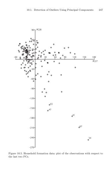
10.1. Detection of Outliers Using Principal Components 24790PC286030-60-3030 60 90 120 150 180PC27-30-60-90-12053-1504741-180-21067-24054-270Figure 10.5. Household formation data: plot of the observations with respect tothe last two PCs.
248 10. Outlier Detection, Influential Observations and Robust EstimationTrace Element ConcentrationsThese data, which are discussed by Hawkins and Fatti (1984), consist ofmeasurements of the log concentrations of 12 trace elements in 75 rock-chipsamples. In order to detect outliers, Hawkins and Fatti simply look at thevalues for each observation on each variable, on each PC, and on transformedand rotated PCs. To decide whether an observation is an outlier, acut-off is defined assuming normality and using a Bonferroni bound withsignificance level 0.01. On the original variables, only two observations satisfythis criterion for outliers, but the number of outliers increases to sevenif (unrotated) PCs are used. Six of these seven outlying observations areextreme on one of the last four PCs, and each of these low-variance PCsaccounts for less than 1% of the total variation. The PCs are thus againdetecting observations whose correlation structure differs from the bulk ofthe data, rather than those that are extreme on individual variables. Indeed,one of the ‘outliers’ on the original variables is not detected by thePCs.When transformed and rotated PCs are considered, nine observations aredeclared to be outliers, including all those detected by the original variablesand by the unrotated PCs. There is a suggestion, then, that transfomationand rotation of the PCs as advocated by Hawkins and Fatti (1984) providesan even more powerful tool for detecting outliers.Epidemiological DataBartkowiak et al. (1988) use PCs in a number of ways to search for potentialoutliers in a large epidemiological data set consisting of 2433 observationson 7 variables. They examine the first two and last two PCs from bothcorrelation and covariance matrices. In addition, some of the variables aretransformed to have distributions closer to normality, and the PCAs are repeatedafter transformation. The researchers report that (unlike Garnham’s(1979) analysis of the household formation data) the potential outliersfound by the various analyses overlap only slightly. Different analyses arecapable of identifying different potential outliers.10.2 Influential Observations in a PrincipalComponent AnalysisOutliers are generally thought of as observations that in some way are atypicalof a data set but, depending on the analysis done, removal of an outliermay or may not have a substantial effect on the results of that analysis.Observations whose removal does have a large effect are called ‘influential,’and, whereas most influential observations are outliers in some respect, outliersneed not be at all influential. Also, whether or not an observation is
- Page 228 and 229: 8.7. Examples of Principal Componen
- Page 230 and 231: 9Principal Components Used withOthe
- Page 232 and 233: 9.1. Discriminant Analysis 201on th
- Page 234 and 235: 9.1. Discriminant Analysis 203Figur
- Page 236 and 237: 9.1. Discriminant Analysis 205Corbi
- Page 238 and 239: 9.1. Discriminant Analysis 207that
- Page 240 and 241: 9.1. Discriminant Analysis 209betwe
- Page 242 and 243: 9.2. Cluster Analysis 211dimensiona
- Page 244 and 245: 9.2. Cluster Analysis 213Before loo
- Page 246 and 247: 9.2. Cluster Analysis 215Figure 9.3
- Page 248 and 249: 9.2. Cluster Analysis 217demographi
- Page 250 and 251: 9.2. Cluster Analysis 219county clu
- Page 252 and 253: 9.2. Cluster Analysis 221choosing a
- Page 254 and 255: 9.3. Canonical Correlation Analysis
- Page 256 and 257: 9.3. Canonical Correlation Analysis
- Page 258 and 259: 9.3. Canonical Correlation Analysis
- Page 260 and 261: 9.3. Canonical Correlation Analysis
- Page 262 and 263: 9.3. Canonical Correlation Analysis
- Page 264 and 265: 10.1. Detection of Outliers Using P
- Page 266 and 267: 10.1. Detection of Outliers Using P
- Page 268 and 269: 10.1. Detection of Outliers Using P
- Page 270 and 271: 10.1. Detection of Outliers Using P
- Page 272 and 273: 10.1. Detection of Outliers Using P
- Page 274 and 275: 10.1. Detection of Outliers Using P
- Page 276 and 277: 10.1. Detection of Outliers Using P
- Page 280 and 281: 10.2. Influential Observations in a
- Page 282 and 283: 10.2. Influential Observations in a
- Page 284 and 285: 10.2. Influential Observations in a
- Page 286 and 287: 10.2. Influential Observations in a
- Page 288 and 289: 10.2. Influential Observations in a
- Page 290 and 291: 10.3. Sensitivity and Stability 259
- Page 292 and 293: 10.3. Sensitivity and Stability 261
- Page 294 and 295: 10.4. Robust Estimation of Principa
- Page 296 and 297: 10.4. Robust Estimation of Principa
- Page 298 and 299: 10.4. Robust Estimation of Principa
- Page 300 and 301: 11Rotation and Interpretation ofPri
- Page 302 and 303: 11.1. Rotation of Principal Compone
- Page 304 and 305: oot of the corresponding eigenvalue
- Page 306 and 307: 11.1. Rotation of Principal Compone
- Page 308 and 309: 11.1. Rotation of Principal Compone
- Page 310 and 311: 11.2. Alternatives to Rotation 279w
- Page 312 and 313: 11.2. Alternatives to Rotation 281F
- Page 314 and 315: 11.2. Alternatives to Rotation 283F
- Page 316 and 317: 11.2. Alternatives to Rotation 285T
- Page 318 and 319: 11.2. Alternatives to Rotation 287T
- Page 320 and 321: 11.2. Alternatives to Rotation 289A
- Page 322 and 323: 11.2. Alternatives to Rotation 291
- Page 324 and 325: 11.3. Simplified Approximations to
- Page 326 and 327: 11.3. Simplified Approximations to
10.1. Detection of Outliers Using <strong>Principal</strong> <strong>Component</strong>s 24790PC286030-60-3030 60 90 120 150 180PC27-30-60-90-12053-1504741-180-21067-24054-270Figure 10.5. Household formation data: plot of the observations with respect tothe last two PCs.


