Jolliffe I. Principal Component Analysis (2ed., Springer, 2002)(518s)

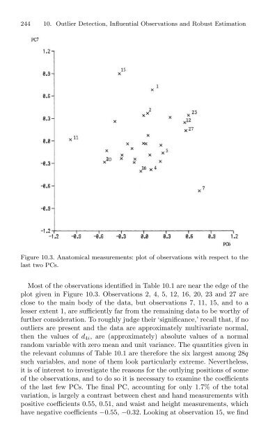
244 10. Outlier Detection, Influential Observations and Robust EstimationFigure 10.3. Anatomical measurements: plot of observations with respect to thelast two PCs.Most of the observations identified in Table 10.1 are near the edge of theplot given in Figure 10.3. Observations 2, 4, 5, 12, 16, 20, 23 and 27 areclose to the main body of the data, but observations 7, 11, 15, and to alesser extent 1, are sufficiently far from the remaining data to be worthy offurther consideration. To roughly judge their ‘significance,’ recall that, if nooutliers are present and the data are approximately multivariate normal,then the values of d 4i , are (approximately) absolute values of a normalrandom variable with zero mean and unit variance. The quantities given inthe relevant columns of Table 10.1 are therefore the six largest among 28qsuch variables, and none of them look particularly extreme. Nevertheless,it is of interest to investigate the reasons for the outlying positions of someof the observations, and to do so it is necessary to examine the coefficientsof the last few PCs. The final PC, accounting for only 1.7% of the totalvariation, is largely a contrast between chest and hand measurements withpositive coefficients 0.55, 0.51, and waist and height measurements, whichhave negative coefficients −0.55, −0.32. Looking at observation 15, we find