Chapter 11. Angular Momentum: General Theory

11. Angular Momentum Theory, November 20, 2009 1Chapter 11. Angular Momentum: General Theory§ 1 Introduction. Angular momentum is intimately related to rotationalmotion of a system of particles. It is essential for understanding the infraredand microwave spectra of a molecule and the properties of the electrons inatoms.Thespinofanelectronorofanucleusisanangularmomentumthathasno classical analog. The spin is accompanied by magnetic moment, whichmeans that we can change the energy of a particle by acting on it with anexternal magnetic field. NMR and ESR spectroscopies are based on thisability. Understanding these extremely rich and important spectroscopictechniques requires a good understanding of angular momentum.In this chapter we define the dynamics of angular momentum throughthe commutation relations between the operators representing its projectionon the coordinate axes. These commutation relations allow us to determinethe eigenstates of the angular momentum operator and derive the matrixrepresentation of the relevant operators. The chapters that follow use thistheory to examine the properties of spin, the orbital angular momentum, andthe angular momentum of more than one particle.§ 2 The definition of the angular momentum operator. In quantum mechanics,we encounter two kinds of angular momenta. The orbital angularmomentum is very similar to the angular momentum in classical mechanics.It describes some aspects of the motion of a particle and it is defined byL = r × p (1)where r is the position of a particle and p is its momentum. To define theoperator ˆ L describing the orbital angular momentum in quantum mechanics,we replace, in Eq. 1, r with ˆr and p with ˆp:ˆL = ˆr × ˆp (2)In addition to the orbital angular momentum, the particles studied inquantum mechanics have an intrinsic angular momentum called spin. Thisis not caused by the motion of the particle (e.g. its rotation); it is insteada property similar to charge or mass. This angular momentum cannot be

11. Angular Momentum Theory, November 20, 2009 2defined by Eq. 2. Born, Heisenberg, and Jordan 1 noted that the angularmomentum defined by Eq. 2 satisfies the commutation relations[ˆL x , ˆL y ]=i¯hˆL z (3)[ˆL y , ˆL z ]=i¯hˆL x (4)[ˆL z , ˆL x ]=i¯hˆL y (5)We take this to be a definition: a vector operator whose components satisfyEqs. 3—5 is an angular momentum. This definition is valid for both theorbital angular momentum and the spin. A compact way of writing theseexpressions, using the Levi-Civitta tensor, is explained in Appendix A11.1. Inthis chapter we will use often a variety of expressions involving commutators;Appendix A11.2 reviews the definition and derives several useful facts.§ 3 ˆL 2 commutes with ˆL x , ˆL y ,andˆL z . We know from classical mechanicsthat the rotational energy is proportional to the square of the angular momentumvector. Since this is an important quantity, we are naturally led toexamine the operatorˆL 2 = ˆL 2 x + ˆL 2 y + ˆL 2 z (6)This operator commutes with ˆL x , ˆL y ,andˆL z .We start with[ˆL z , ˆL 2 ]=[ˆL z , ˆL 2 x]+[ˆL z , ˆL 2 y]+[ˆL z , ˆL 2 z] (7)Any operator commutes with a power of itself, so[ˆL z , ˆL 2 z]=0 (8)To calculate [ ˆL 2 x, ˆL z ], we use the relationship, derived in Appendix A11.2(Eq. 160),[Â, ˆB 2 ]=[Â, ˆB] ˆB + ˆB[Â, ˆB],giving us[ˆL z , ˆL 2 x]=[ˆL z , ˆL x ]ˆL x + ˆL x [ˆL z , ˆL x ], (9)1 M. Born, W. Heisenberg, and P. Jordan, Zur Quantenmechanik II, Zeitschrift fürPhysik 35 (8—9), 557-615 (published August 1926; received November 16, 1925). Englishtranslation in: B. L. van der Waerden, editor, Sources of Quantum Mechanics (DoverPublications, 1968, ISBN 0-486-61881-1).

11. Angular Momentum Theory, November 20, 2009 3followed by Eq. 5, to obtain[ˆL z , ˆL 2 x ]=i¯hˆL y ˆLx +i¯hˆL x ˆLy =i¯h ˆLy ˆLx + ˆLx ˆLyYou can show similarly that[ˆL z , ˆL 2 y]=−i¯h ˆLy ˆLx + ˆLx ˆLyUsingEqs.8—11inEq.7gives(10)(11)Inthesameway,youcanshowthat[ˆL 2 , ˆL z ]=0 (12)[ˆL 2 , ˆL x ]=0 (13)and[ˆL 2 , ˆL y ]=0 (14)Common sense tells us that if Eq. 12 is true, then Eqs. 13 and 14 must alsobe true, because there is no physical agent that differentiates between theOZandOXorOYdirections.§ 4 The eigenstates of ˆL 2 and ˆL z . Since ˆL 2 commutes with ˆL z , there existsa set of eigenfunctions of ˆL 2 that are also eigenfunctions of ˆL z .BecauseˆL zdoes not commute with ˆL x or with ˆL y , a joint eigenstate of ˆL 2 and ˆL z cannotbe an eigenstate of ˆL y or of ˆL z .Let us examine in more detail what this means. Since ˆL 2 and ˆL z commute,there exists a set of kets |L z ; α, β that satisfy the eigenvalue equations forthose two operators:ˆL 2 |L z ; α, β = α|L z ; α, β (15)ˆL z |L z ; α, β = β|L z ; α, β (16)α is the value that L 2 can have in a measurement. It is therefore relatedto the rotational energy. β is the value that the projection of the angularmomentum on the Z-axis can take. The symbol L z inside the ket reminds usthat this is an eigenket of ˆL z ,notofˆL x or ˆL y .But ˆL 2 also commutes with ˆL x , so there must exist a set of kets |L x ; α, βsuch thatˆL 2 |L x ; α, β = α|L x ; α, β (17)ˆL x |L x ; α, β = β|L x ; α, β (18)

11. Angular Momentum Theory, November 20, 2009 4As long as no electric or magnetic field acts on the system there is no physicaldifference between the OX and the OZ axes. Therefore, the values that βcan take in |L x ; α, β are the same as the values it can take in |L z ; α, β.In what follows, we concentrate on the joint eigenstates of ˆL 2 and ˆL z .Atthis point there is no reason to prefer ˆL z over ˆL x or ˆL y .Suppose that we have performed an experiment that places the systemin the state |L z ; α, β. We can measure L 2 and get the value α, orwecanmeasure L z and get the value β. However, if we measure L x , when the systemis in state |L z ; α, β, wefind L x to be β with the probability|L x ; α, β | L z ; α, β| 2When the system is in the state |L z ; α, β, weknowL 2 and L z with certaintybut we only know the probability that L x takes a given value. For someonefamiliar with quantum mechanics, this is not surprising. ˆLz and ˆL x do notcommute so the eigenstate |L z ; α, β cannot be an eigenstate of ˆL x .These results are incomprehensible within classical physics, where thereis no physical law to prevent us from knowing with certainty all three projectionsof any vector once we know the state of the system (i.e. the valuesof the position and of the momentum).§ 5 ˆL 2 and ˆL z commute with other operators. One difficulty in graspingthe physics of angular momentum comes from the fact that in many concreteproblems, ˆLx , ˆLy ,andˆL z are not the only operators describing thesystem. For example, we might examine two particles interacting through acentral force. This means that the potential energy V (r) depends only onthe distance r between the particles and is independent of their orientationin space. You know two examples of such systems: the hydrogen atom andthediatomicmolecule.The eigenvalue problem for the Hamiltonian of the hydrogen atom is (seeMetiu, Quantum Mechanics, p.206)− ¯h22μ1r 2∂r 2 ∂ψ ∂r ∂r+ ˆL 2ψ + V (r)ψ = Eψ (19)2μr2 We see that besides the angular momentum squared ˆL 2 , the equation containsthe potential energy V (r) and the radial kinetic energy (the first term).You have also learned that the Hamiltonian Ĥ of the hydrogen atom commuteswith ˆL 2 and with ˆL z . This means that Ĥ, ˆL 2 ,andˆL z have common

11. Angular Momentum Theory, November 20, 2009 5eigenstates, denoted by |n, j, m.atom is (see Metiu, p. 300)In the state |n, j, m, the energy of thethe square of the angular momentum isE n = − μe2 z 22(4π 0 ) 2¯h 2 1n 2 , (20)¯h 2 j(j +1), (21)and the projection of the angular momentum on the z-axis isIn other words, we have¯hm (22)Ĥ|n, j, m = − μe2 z 2 12(4π 0 ) 2¯h 2 |n, j, mn2 (23)ˆL 2 |n, j, m =¯h 2 j(j +1)|n, j, m (24)ˆL z |n, j, m =¯hm|n, j, m (25)Here j indicates the eigenvalue of ˆL 2 and m indicates the eigenvalue of ˆL z .We learn from this example that the eigenstates of ˆL 2 and ˆL z may also beeigenstates of other observables that commute with ˆL 2 and ˆL z (in this case,the energy). These eigenstates are labeled by additional quantum numbers(n, inthiscase);theyare|n, j, m, notjust|j, m.A similar situation appears in the case of the diatomic molecules. If wemake the rigid-rotor approximation and the harmonic approximation, theeigenvalue equation for the energy, Eq. 19 becomes (see Metiu, Chapter 16)− ¯h22μ1r 2∂r 2 ∂ψ + ˆL 2ψ + 1 ∂r ∂r 2μr02 2 k(r − r 0) 2 ψ = Eψ (26)The eigenstates are |ψ = |v, j, m, in which the molecule has the vibrationalenergyE v =¯hω v + 1 (27)2and the values of ˆL 2 and ˆL z given by Eqs. 21 and 22. Eqs. 24 and 25 holdfor this example also.

11. Angular Momentum Theory, November 20, 2009 6In general, when ˆL 2 and ˆL z commute with other operators, their eigenstatesmust be eigenstates of those operators. When we need to make thisexplicit, these eigenstates will be labeled |a, j, m, wherea tells us the valuethat the quantities represented by these other operators takes, when thesystem is in a pure state |a, j, m and a measurement is made.§ 6 A more convenient notation. I now change notation by writingThe eigenvalue equations Eqs. 15 and 16 becomeα =¯h 2 j(j +1) (28)β =¯hm (29)|L z ; α, β = |L z ; j, m (30)ˆL 2 |L z ; j, m =¯h 2 j(j +1)|L z ; j, m (31)andˆL z |L z ; j, m =¯hm|L z ; j, m (32)Setting α =¯h 2 j(j + 1) needs further examination. We must haveα ≥ 0 (33)because α is a value that L 2 can take. It is a minor complication that theequation α =¯h 2 j(j + 1) has two solutions for j:j 1 = − 1 1+1+4α/¯h 2 (34)2andj 2 = 1 2−1+1+4α/¯h 2(35)Because α/¯h 2 ≥ 0, both roots j 1 and j 2 are real, j 1 is negative, and j 2 is nonnegative.Remember that α is a physical observable while j is an arbitrarymathematical quantity introduced for convenience. You can verify that thenegative values of j give the same values of α as the non-negative ones. Wecan choose either for indexing the kets, and we choosej ≥ 0 (36)Note also that m must be a real number (¯hm is a value of L z ). BecauseL z is equally likely to be positive or negative, we expect m to be able to take

11. Angular Momentum Theory, November 20, 2009 7both positive and negative values. Moreover, we guess that if m is an allowedvalue, then −m is also allowed since the projection of the angular momentumvector on the OZ axis can be oriented along OZ (m >0) or opposite to it(m

11. Angular Momentum Theory, November 20, 2009 8Our strategy relies on commutation relations and I derive here all thecommutations relations that we need. The commutators of ˆL + and ˆL − withˆL 2 and ˆL z are easily derived from the definitions, Eqs. 37 and 38, and theoriginal commutation relations, Eqs. 3—5. They are[ˆL z , ˆL + ]=¯hˆL + (41)and[ˆL z , ˆL − ]=−¯hˆL − (42)We also have[ˆL 2 , ˆL + ]=[ˆL 2 , ˆL − ]=0 (43)because ˆL 2 commutes with both ˆL x and ˆL y , hence with both ˆL + and ˆL − .To carry out our program of determining what happens when ˆL + and ˆL −act on |L z ; j, m, weneedtofind expressions that contain ˆL + and/or ˆL − inthe left-hand side and only ˆL z and ˆL 2 in the right-hand side. I derive belowseveral such expressions. One of them isˆL − ˆL+ = (ˆL x − iˆL y )(ˆL x +iˆL y ) (used Eqs. 37&38)= ˆL 2 x + ˆL 2 y +i(ˆL x ˆLy − ˆL y ˆLx )= ˆL 2 x + ˆL 2 y +i[ˆL x , ˆL y ]= ˆL 2 x + ˆL 2 y +i 2¯hˆL z (used Eq. 3)= ˆL 2 − ˆL 2 z − ¯hˆL z (used ˆL 2 = ˆL 2 x + ˆL 2 y + ˆL 2 z) (44)SimilarlyWe can add Eqs. 44 and 45 to obtainˆL + ˆL− = ˆL 2 − ˆL 2 z +¯hˆL z (45)Usingandwe can rewrite Eq. 46 asˆL + ˆL− + ˆL − ˆL+=2− ˆL 2 z (46)ˆL † + = ˆL − (47)ˆL † − = ˆL + (48)ˆL † − ˆL − + ˆL † + ˆL +2= ˆL 2 − ˆL 2 z (49)

11. Angular Momentum Theory, November 20, 2009 9§ 9 Find expressions for ˆL + |L z ; j, m and ˆL − |L z ; j, m. For notationalconvenience, I will drop the marker L z from the eigenkets |L z ; j, m andreinstate it only when there is some possibility of confusion.The fact that ˆL 2 and ˆL + commute leads toˆL 2 ˆL+ |j, m = ˆL ˆL2 + |j, m =¯h 2 j(j +1)ˆL + |j, m (50)This equation tells us that if |j, m is an eigenstate of ˆL 2 with the eigenvalue¯h 2 j(j +1) then ˆL + |j, m is also an eigenstate of ˆL 2 , with the same eigenvalue¯h 2 j(j +1).Since [ˆL z , ˆL + ]=¯hˆL + (Eq. 41), we haveˆLz ˆL+ − ˆL + ˆLz|j, m =¯hˆL+ |j, m (51)Use ˆL z |j, m =¯hm|j, m in the left-hand side and rearrange the terms:ˆL zˆL+ |j, m =¯h(m +1) ˆL+ |j, m (52)Eq. 52 tells us that ˆL + |j, m is either zero, which is uninteresting, or it is aneigenstate of ˆL z with the eigenvalue ¯h(m +1). ThismeansthatˆL + |j, m = C + (j, m)|j, m +1 (53)where C + (j, m) isanumberthatmayormaynotdependonj and m.Note that in Eq. 53, ˆL + acts on |j, m and does not affect the value of jbut changes m. This is in agreement with Eq. 50, which says that ˆL + |j, mis an eigenfunction of ˆL 2 with the eigenvalue ¯h 2 j(j +1).A similar argument starts from [ˆL z , ˆL − ]=−¯hˆL − (Eq. refeq11:3.11.4) andconcludes thatˆL − |j, m = C − (j, m)|j, m − 1 (54)where C − (j, m) is another, unknown constant. Also, ˆL − |j, m is an eigenfunctionof ˆL 2 corresponding to the eigenvalue ¯h 2 j(j +1).The operators ˆL + and ˆL − are called ladder operators; ˆL + is called a raisingoperator and ˆL − ,alowering operator. When ˆL + acts on |j, m, itincreasesm by 1 and multiplies the result by C + (j, m); when ˆL − acts on |j, m, itdecreases m by 1 and multiplies the result by C − (j, m). The operators ˆL +and ˆL − do not affect j in |j, m, becausebothˆL + and ˆL − commute with ˆL 2and therefore they have common eigenstates with ˆL 2 . In other words, theymust convert a state in which ˆL 2 has the value ¯h 2 j(j + 1) into a state inwhich ˆL 2 has thesamevalue¯h 2 j(j +1).

11. Angular Momentum Theory, November 20, 2009 10§ 10 The constants C + (j, m) and C − (j, m). To determine C + (j, m) orC − (j, m), we need to derive first a few helpful results. Consider|λ = Â|x (55)where |x is an arbitrary ket and  is an arbitrary operator. We haveλ | λ = Âx | Âx = x | †  | x (56)I used here the property Âx | z = x | † z of adjoint operators (|x and |zare arbitrary kets).In addition, ifÂ|x = a|y (57)where a is a number, thenλ | λ = ay | ay = a ∗ ay | y (58)Let us use Eqs. 56 and 58 to determine C + . To do this I apply Eq. 56 toand obtainWe also haveNowapplyEq.58toget|λ ≡ˆL + |j, m (59)λ | λ = j, m | ˆL † + ˆL + | j, m (60)λ = ˆL + |j, m = C + |j, m +1 (61)λ | λ = C ∗ +C + j, m +1| j, m +1 = C ∗ +C + (62)I used the fact that j, m +1| j, m +1 = 1 (or, if |j, m +1 is zero, then sois C + ). The two expressions for λ | λ must be equal and thereforej, m | ˆL † + ˆL + | j, m = C ∗ + C + (63)I am very pleased with this equation, for two reasons. First, I obtainedaformulaforC + . Second, this equation contains ˆL + ˆL− ,which,accordingtoEq. 44 isˆL + ˆL− = ˆL 2 − ˆL 2 z − ¯hˆL z

11. Angular Momentum Theory, November 20, 2009 11This expresses ˆL + ˆL− in terms of ˆL 2 and ˆL z . I know how ˆL 2 and ˆL z act on|j, m and therefore I can readily calculate the matrix element in Eq. 63.Eq. 63 determines the absolute value of C + but not its phase. Since allphysical properties of a ket are independent of a phase factor in front of it,IcantakeinC + anyphaseIwant.IchooseitsothatC + (j, m) = j, m | ˆL † ˆL + + | j, m (64)Now use Eq. 44 in Eq. 64:C + (j, m) = j, m | ˆL2 − ˆL 2z − ¯hˆL z | j, m (65)Using the eigenvalue equations for ˆL 2 and ˆL z (Eqs. 31—32), we rewrite Eq. 65asC + (j, m) =¯h j(j +1)− m(m +1) (66)(we used j, m | j, m =1).Finally, putting C + (j, m) given by Eq. 66 into Eq. 53 givesˆL + |j, m =¯h j(j +1)− m(m +1)|j, m +1 (67)Note that ˆL + |j, m is an eigenstate of ˆL 2 corresponding to the eigenvalue¯hj(j + 1) and an eigenstate of ˆL z corresponding to the eigenvalue (m +1)¯h.However, |j, m is not an eigenstate of ˆL + . It should not be, because ˆL +does not commute with ˆL 2 or with ˆL z .To calculate C − (j, m), we follow the reasoning used to find C + (j, m). Thisleads toC − (j, m) =¯h j(j +1)− m(m − 1) (68)andˆL − |j, m =¯h j(j +1)− m(m − 1) |j, m − 1 (69)We can now calculate (use Eqs. 66, 69, 39)ˆL x |j, m = 1 2 (ˆL + + ˆL − )|j, mSimilarly (use Eqs. 66, 69, 40)= 1 2 [C +(j, m)|j, m +1 + C − (j, m)|j, m − 1] (70)ˆL y |j, m = 1 2i [C +(j, m)|j, m +1−C − (j, m)|j, m − 1] (71)

11. Angular Momentum Theory, November 20, 2009 12§ 11 The matrix elements of ˆL + , ˆL − , ˆL x , ˆL y in the basis set |j, m. Nowthat we know how ˆL + and ˆL − act on |j, m (Eqs. 67 and 69), we can calculatethe matrix elementsj ,m | ˆL+ | j, m = ¯h j(j +1)− m(m +1)j ,m | j, m +1= ¯h j(j +1)− m(m +1)δ j jδ m ,m+1 (72)The only non-zero matrix elements are those for which m = m+1 and j = j.Therefore onlyj, m +1| ˆL+ | j, m =¯h j(j +1)− m(m +1) (73)differs from zero.The matrix elements of ˆL − arej ,m | ˆL− | j, m =¯h j(j +1)− m(m − 1) δ j jδ m ,m−1 (74)and onlyj, m − 1 | ˆL− | j, m =¯h j(j +1)− m(m − 1) (75)differs from zero.Since(seeEq.39)ˆL x = ˆL + + ˆL −2we havej ,m | ˆL x | j, m = ¯h 2 (C +(j, m) δ j jδ m ,m+1 + C − (j, m) δ j jδ m ,m−1) (76)Only the matrix elementsj, m +1| ˆL x | j, m = ¯h 2 C +(j, m) (77)andj, m − 1 | ˆL x | j, m = ¯h 2 C −(j, m) (78)differ from zero.Using (see Eq. 40)ˆL y = ˆL + − ˆL −2i

11. Angular Momentum Theory, November 20, 2009 13with Eqs. 72 and 74 leads toj ,m | ˆL y | j, m = ¯h 2i (C +(j, m) δ j jδ m ,m+1 − C − (j, m) δ j jδ m ,m−1) (79)Only the matrix elementsj, m +1| ˆL y | j, m = ¯h 2i C +(j, m) (80)andj, m − 1 | ˆL y | j, m = − ¯h 2i C −(j, m) (81)differ from zero.This covers all the matrix elements used in applications. However, westill don’t know what values j and m can take, since we do not know theeigenvalues of ˆL 2 and ˆL z . Next, we start working to find them.The values of j and mWe have decided to use the eigenstates |j, m of ˆL 2 and ˆL z as a basis setfor other operators relevant to angular momentum, and we have managedto calculate their matrix elements. The remaining task is to determine theallowed values of j and m.§ 12 For a given j, m has a highest and a lowest value. A classical interpretationof angular momentum tells us that if ˆL 2 is fixed then ˆL z must havean upper and a lower bound. Indeed the projection of a vector on an axiscanatmostbeequaltothelength of the vector: the projection has theupper bound and the lower bound −. Since quantum mechanics is notclassical mechanics, it will be reassuring to prove that, for a given j, m hasan upper and a lower bound.Recall that (Eqs. 46 and 49)andˆL + ˆL− + ˆL − ˆL+2ˆL † − ˆL − + ˆL † + ˆL +2= ˆL 2 − ˆL 2 z (82)= ˆL 2 − ˆL 2 z (83)

11. Angular Momentum Theory, November 20, 2009 14From properties of the inner product, we know that for any ket |x andany operator Â, wehavex | †  | x ≥0 (with equality only when Â|x =0).Taking the matrix element of the operator in Eq. 83 with the non-zero ket|j, m givesj, m | ˆL † − ˆL − | j, m + j, m | ˆL † + ˆL + | j, m =2¯h 2 (j(j +1)− m 2 ) (84)Since the left-hand side cannot be negative, we conclude thatj(j +1)− m 2 ≥ 0 (85)This means that if j is fixed then m hasbothalowerboundandanupperbound. We don’t know what the bounds are but we know that they exist, solet us denote them by m and m u .This gives us two new equations to play with:ˆL + |j, m u = 0 (86)ˆL − |j, m = 0 (87)To derive them, observe that, according to Eq. 53, ˆL + |j, m u = C + (j, m u )|j, m u +1. Since no value of m can be larger than m u ,thestate|j, m u +1 cannotexist and the ket is zero (which proves Eq. 86). One arrives at Eq. 87similarly.Now let us act with ˆL − on Eq. 86 and with ˆL + on Eq. 87, to obtainWhy do I do that? Because we know that (Eq. 44)ˆL − ˆL+ |j, m u = 0 (88)ˆL + ˆL− |j, m = 0 (89)ˆL − ˆL+ = ˆL 2 − ˆL 2 z − ¯hˆL z ;the right-hand side of this equation contains only operators that act on |j, maccording to known rules, which means that we can calculate0 = ˆL − ˆL+ |j, m =(ˆL 2 − ˆL 2 z − ¯hˆL z )|j, m= (¯h 2 j(j +1)− ¯h 2 m 2 u − ¯h2 m u )|j, m u (90)This implies thatj(j +1)− m 2 u − m u =0 (91)

11. Angular Momentum Theory, November 20, 2009 15Similarly, using (see Eq. 45)in Eq. 89 givesˆL + ˆL− = ˆL 2 − ˆL 2 z +¯hˆL zj(j +1)− m 2 + m =0 (92)Solving Eq. 92 for j(j + 1) and using the result in Eq. 91 givesThis equation has two solutionsandm u (m u +1)=m (m − 1) (93)m u = −m (94)m u = m − 1 (95)The second root is excluded by the fact that m u ≥ m by definition.Weseethereforethatm u = −m . Symmetry requires the possible projectionsof ˆL along OZ to be equal to and of opposite sign to the possibleprojections in the direction opposite to OZ. Eq. 94 agrees with this requirement.§ 13 The values of m and j. We have learned a lot but we still don’t knowwhich values j and m can take. Here we settle this question.Letusconsideraket|j, m 0 where m 0 is an allowed value of m for thegiven j. Acting on that ket with ˆL + repeatedly, we obtainˆL + |j, m 0 = C + (j, m 0 )|j, m 0 +1,ˆL 2 + |j, m 0 = C + (j, m 0 )C + (j, m 0 +1)|j, m 0 +2,etc. After some number n u of steps, this procedure must generate a ketproportional to |j, m u . If it did not, then we could apply ˆL + indefinitely,which contradicts the fact that m has a largest value, namely m u . Thereforewe must havem u = m 0 + n u (96)where n u is a non-negative integer. Similarly, applying ˆL − to |j, m 0 some n times produces a ket proportional to |j, m ,sothatm = m 0 − n (97)

11. Angular Momentum Theory, November 20, 2009 16with n a non-negative integer. From Eqs. 96 and 97, it follows thatm u − m =(m 0 + n u ) − (m 0 − n )=n u + n ≡ n (98)where n is a non-negative integer. Since we already know that m u = −m (Eq. 94), we conclude that2m u = n (99)We also know that (see Eq. 91)This has two solutionsj(j +1)=m 2 u + m u = m u (m u + 1) (100)j = m u (101)andj = −m u − 1 (102)Eq. 102 is not compatible with the facts that m u ≥ 0andj ≥ 0, so we caneliminate it as irrelevant.Now combining m u = n/2 (Eq. 99) with Eq. 101 givesj = n 2(103)We have obtained a startling result: j can be either a non-negative integer(if n iseven)orahalf-integer(ifn is odd). In addition, the largest value ofm is j and (since m = −m u ) the smallest value of m is −j. Therefore mcan take the 2j +1values−j, −j +1,..., j − 1, j.The theory of orbital angular momentum (see Metiu, Chapter 14, p. 220ff),basedontheequation L = r × p, tells us that half-integer values of j are notallowed for orbital angular momentum. However, by using the commutationrelations to define the angular momentum, we have found that j can be eitherinteger or half-integer. We know of no additional condition that we canuse to conclude that half-integers are not allowed in general. Therefore thepostulate that the electron has an intrinsic angular momentum (the spin)with j =1/2 is in harmony with conclusions derived from the commutationrelations.§ 14 Summary. This lengthy derivation led us to the following results. ˆL2and ˆL z have common eigenstates |ˆL z ; j, m for whichˆL 2 |ˆL z ; j, m =¯h 2 j(j +1)|ˆL z ; j, m (104)

11. Angular Momentum Theory, November 20, 2009 17andˆL z |ˆL z ; j, m =¯hm |ˆL z ; j, m. (105)j can be either a non-negative integer or a positive half-integer (that is, ofthe form integer/2). m can take 2j + 1 discrete valuesm = −j, −j +1, −j +2,...,j− 2,j− 1,j (106)For example, if j = 3 then m can take 2 × 3 +1=4values,namely2 2m = − 3 2 , −3 2 +1, 32 − 1, 32 = −3 2 , −1 2 , 12 , 32If j =3thenm takes the 2 × 3+1=7values−3, −2, 1, 0, 1, 2, 3.We have also found thatandˆL x |ˆL z ; j, m = 1 2 [C +(j, m)|ˆL z ; j, m +1 + C − (j, m)|ˆL z ; j, m − 1] (107)ˆL y |ˆL z ; j, m = 1 2i [C +(j, m)|ˆL z ; j, m +1−C − (j, m)|ˆL z ; j, m − 1] (108)withC + (j, m) =¯h j(j +1)− m(m + 1) (109)andC − (j, m) =¯h j(j +1)− m(m − 1). (110)Note that |j, m =0ifm ∈ [−j, j].The matrix elements needed in computations areˆL z ; j ,m | ˆL z | ˆL z ; j, m = δ jj δ mm ¯hm (111)ˆL z ; j ,m | ˆL 2 | ˆL z ; j, m = δ jj δ mm ¯h 2 j(j + 1) (112) ˆL z ; j ,m | ˆL x | ˆLC+ (j, m)δ mz ; j, m = δ ,m+1 + C − (j, m)δ m ,m−1jj (113)2 ˆL z ; j ,m | ˆL y | ˆLC+ (j, m)δ mz ; j, m = δ ,m+1 − C − (j, m)δ m ,m−1jj (114)2iNote that all these matrix elements are zero if j = j . This means thatin the basis set |ˆL z ; j, m, the matrices of ˆLx and ˆL y consist of smallermatrices strung along the diagonal; there are no non-zero matrix elementsj, m | Ôj ,m in which j = j if Ô = ˆL x , ˆL y , ˆL + , or ˆL − or any function ofthem.

11. Angular Momentum Theory, November 20, 2009 18The eigenvalue problems for angular momentum operators§ 15 Introduction. We have seen several times that kets are very useful fortheoretical analysis, but practical calculations often use the representation ofkets by vectors and of operators by matrices. In this section I review brieflythe general theory and then apply it to the case of j = 3 as an example.Let us assume that on physical grounds we have decided that a certainphysical system can be described by a ket space generated by the orthonormalbasis set |η 1 , |η 2 , ..., |η N . An arbitrary state |ψ is then represented as|ψ =N|η i η i | ψ ≡i=1and an arbitrary operator Ô byÔ =Ni=1 k=1N|η i η i | Ô | η kη k | ≡N|η i c i (115)i=1Ni=1 k=1N|η i O ik η k | (116)Sinceweareassumedtoknow|η i , i =1, 2,...,N, knowing the vectorψ = {c 1 ,c 2 ,...,c N } (117)is equivalent to knowing |ψ (because of Eq. 115). Eq. 116 tells us that weknow how to operate with Ô if we know the matrix elementsO ik ≡η i | Ô | η k (118)The basis set kets |η i are represented by the vectorsη 1 = {1, 0,...,0}.η N = {0, 0,...,1}⎫⎪⎬⎪⎭(119)and thereforeNψ = c i η i (120)i=1The eigenvalue problem Ô|ψ = o|ψ is represented by the eigenvalue problemfor the matrix OO ik c k = oc i ,k

11. Angular Momentum Theory, November 20, 2009 20• j =0,m=0• j =1,m= −1• j =1,m=0• j =1,m=1• etc.The state with j = 0 generates a 1 × 1 block, the states with j = 1 generatea3× 3 block, . . . ; in general, the states having an arbitrary j generate a(2j +1)× (2j + 1) block. This break-up into blocks makes this basis setparticularly simple to use in calculations. Physically it signifies that stateswith different values of j are not coupled by any of the operators ˆL 2 , ˆL z , ˆL x ,and ˆL y .Because of this “block” property, we can treat physical problems involvingaspecific j within a reduced space generated by the basis set|j, −j, |j, −j +1, ..., |j, j − 1, |j, j (125)§ 17 The case j =1. Let us solve some problems for j =1. Thebasissetis|1, −1, |1, 0, |1, 1 (126)Since we know that j =1,thefirst index is superfluous and we use insteadthe notation | − 1, |0, |1. The matrix representing an operator Ô in thissubspace is⎛⎞−1 | Ô | − 1 −1 | Ô | 0 −1 | Ô | 1O = ⎜⎝ 0 | Ô | − 1 0 | Ô | 0 0 | Ô | 1 ⎟⎠ (127)1 | Ô | − 1 1 | Ô | 0 1 | Ô | 1A look at Eqs. 111 and 112 tells us that the matrix elements 1,m| ˆL 2 | 1,m and 1,m| ˆL z | 1,m are zero if m = m . Therefore the corresponding matricesare diagonal:⎛L 2 =¯h 2 ⎜(1)(1 + 1) ⎝1 0 00 1 00 0 1⎞⎟⎠ (128)

11. Angular Momentum Theory, November 20, 2009 21and⎛⎜L z = ⎝−¯h 0 00 0 00 0 ¯h⎞⎟⎠ (129)No surprise here. The basis set consists of eigenstates |j, m of ˆL 2 and ˆL zand therefore the matrices of these operators, in that basis set, are diagonaland the diagonal elements are the eigenvalues of the operator.The matrices corresponding to ˆL x and ˆL y are more interesting. Let uslook at ˆL x , and use Eq. 113 together with Eqs. 109 and 110. I calculate, asan example, −1 | ˆL x | − 1. Wehavebecause (see Eq. 113)andAnother example is (use Eq. 113)m = −1 | ˆL x | m = −1 =0 (130)δ m ,m+1 = δ −1,−1+1 = δ −1,0 =0δ m ,m−1 = δ −1,−1−1 = δ −1,−2 =0m = −1 | ˆL x | m =0 = C +(1, 0)δ −1,0+1 + C − (1, 0)δ −1,0−12= C −(1, 0)2(131)withTogether these giveC − (1, 0) = ¯h 1(1 + 1) − 0(0 − 1) = ¯h √ 2 (132)−1 | ˆL x | 0 = ¯h √2(133)Patiently calculating all the matrix elements leads to 2⎛⎞¯h0 √2 0¯h√ ¯h20 √2L x =⎜⎝0¯h √2 0⎟⎠ (134)2 The top row is m = −1, the middle row is m = 0, and the bottom row is m =1;the left column is m = −1, the middle column is m = 0, and the right column is m =1.In all entries j =1.

11. Angular Momentum Theory, November 20, 2009 22ThesematrixelementswerecalculatedinWorkBook11.Angular Momentum.nb.The matrix must be Hermitian because ˆL x represents an observable, andtherefore we need only calculate the matrix elements in the lower-left triangle;the ones in the upper-right triangle are then obtained from m | Ô | m =m | Ô | m ∗ . In addition, the δs in Eq. 113 tell us that the diagonal elements(that is, those with m = m) are zero and that in the lower-left triangle, only0 | ˆL x | − 1 and 1 | ˆL x | 0 are nonzero.Exercise 1 Show that for j =1Is the matrix Hermitian?L y =¯h √2⎛⎜⎝0 −i 0i 0 −i0 i 0⎞⎟⎠ (135)Exercise 2 Verify that the matrices representing the operators satisfy thecommutation relationsand thatL x L y − L y L x =i¯hL zL y L z − L z L y =i¯hL xL z L x − L x L z =i¯hL yL 2 = L 2 x + L 2 y + L 2 z§ 18 The eigenvalues and eigenvectors of ˆL x for j = 1. Now that wehave a matrix representation of ˆL x , we can calculate the eigenvalues andeigenvectors of this operator. We need to know them because they appearin some problems in spectroscopy. I solved the eigenvalue problem in Cell 6of the Mathematica file WorkBook11. Angular momentum.nb. Theresultsare (Cell 6 of WorkBook11):eigenvalue eigenvector−¯h { 1, − √ 1 12 2, } 20 {− √ 1 12, 0, √2 }¯h { 1, √2 1 1, }2 2

11. Angular Momentum Theory, November 20, 2009 23The eigenvectors are normalized. I remind you that in this basis set theeigenvectors of L z are {1, 0, 0}, {0, 1, 0}, and{0, 0, 1}.WearepleasedtoseethatL x has the same eigenvalues as L z . Since noforce that breaks spherical symmetry acts on the system, there is no preferreddirection in space. The possible values of the projection of the vector L onthe x-axis must be the same as those of the projection on the z-axis.Exercise 3 Show that L y has the same eigenvalues as L z .6)The eigenstates of ˆL x in the basis set |L z ;1,m are (see WorkBook11, Celleigenvalueeigenket−¯h |L x ;1, −1 = 1 2 |L z;1, −1− 1 √2|L z ;1, 0 + 1 2 |L z;1, 1 (136)0 |L x ;1, 0 = − 1 √2|L z ;1, −1 + 1 √2|L z ;1, 1 (137)¯h |L x ;1, 1 = 1 2 |L z;1, −1 + 1 √2|L z ;1, 0 + 1 2 |L z;1, 1 (138)I have had to augment the notation with a new index: |L z ; j, m are eigenketsof ˆL z ,and|L x ; j, m are those of ˆL x .If we manage to place the system in the state |L x ;1, −1, ameasurementof L x is guaranteed to give the result −¯h. However, if we measure L z ,when the system is in the state |L x ;1, −1, we obtain the value −¯h with theprobabilityP −1 ≡ |L z ;1, −1 | L x ;1, −1| 2 12 L z;1, −1 | L z ;1, −1−√ 1 L z ;1, −1 | L z ;1, 0 + 1 22 2 L z;1, −1 | L z ;1, 1== 1 4(139)To get this, I used the orthonormality condition L z ;1,m| L z ;1,m = δ mm .Similarly, the probability P 0 that L z is zero is given byP 0 ≡ |L z ;1, 0 | L x ;1, −1| 2 = 1 2(140)

11. Angular Momentum Theory, November 20, 2009 24and the probability P 1 that L z is 1 byP 1 ≡ |L z ;1, 1 | L x ;1, −1| 2 = 1 4(141)P −1 + P 0 + P 1 =1,whichisamust.This result is consistent with the fact that ˆL z does not commute withˆL x and therefore there is no state in which the value of both is known withcertainty.We can also calculate the average value of L z ,L z ≡L x ;1, −1 | ˆL z | L x ;1, −1when the system is in the state |L x ;1, −1. Using Eq. 136 in the right-handside (for |L x ;1, −1) givesL x ;1, −1 | ˆL z | L x ;1, −1 = L x ;1, −1 | ˆL 1z | L z ;1, −12 −L x ;1, −1 | ˆL 1√2z | L z ;1, 0+ L x ;1, −1 | ˆL 1z | L z ;1, 12UsingEq.136again,aswellasL z ; j, m | ˆL z | L z ; j, m = δ mm ¯hm, leadstoL z =This is the same as 1 1 1√2 1 1(−¯h) − (0) + (¯h) =0 (142)22221L z =m=−1¯hmP m =(−¯h) 1 4 +(0)1 2 +(¯h)1 4=0, (143)as it should be This result is physically reasonable. Since no forces breakspherical symmetry, there is no bias to prefer positive values of L z overnegative values. The average is zero because the value −¯h is as probable as¯h.§ 19 The energy of the electron in the hydrogen atom exposed to a magneticfield. When we discuss the hydrogen atom, I will show that when the atom

11. Angular Momentum Theory, November 20, 2009 25is exposed to a magnetic field B, the energy of its electron changes. TheHamiltonian isĤ = Ĥ0 +e ˆL · B (144)2m ewhere m e is the mass of the electron, e is the proton charge, and Ĥ0 is theHamiltonian of the atom in the absence of the field.I am ignoring other terms in the Hamiltonian since I only want to illustratehow we handle this kind of problem. The question is: what happens tothe energy of the electron when it is exposed to the magnetic field? I answerfirst the question for the case when I was smart enough to pick the z-axisalong B. InthiscaseB = {0, 0,B} and ˆ L · B = ˆLz . The Hamiltonian isĤ = Ĥ0 +e2m eˆLz B,where B is the magnitude of the field B. Since ˆL z and Ĥ0 commute, theyhave joint eigenstates, denoted by |n, j, m, wheren gives the energy E n inthe absence of the field.I want to know what happens to the energy of the states |2,j,m whenthe field is on. To answer this question, I will use these states as a basis set.Therefore I haveĤ|n, j, m = Ĥ0|n, j, m + eB ˆLz |n, j, m2m e= E n + eB m |n, j, m (145)2m eWe see that |n, j, m are eigenstates of the Hamiltonian defined by Eq. 144.The energy spectrum is given byE n + eB2m em (146)As noted above, E n is the energy of the atom in the absence of the field:E n = − Ryn 2 , (147)where Ry is the Rydberg constant. For the case n = 2, in the absence of thefield, the atom has four degenerate states: |2, 0, 0, |2, 1, −1, |2, 1, 0, and

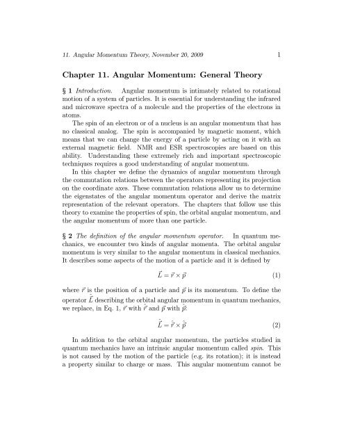
11. Angular Momentum Theory, November 20, 2009 26|2, 1, 1. Ifthefield is on, the energy of these states changes to that given byEq. 146 and depends on the quantum number m. The states arestate |n, j, m energy change|2, 0, 0 −Ry/4 unchanged|2, 1, −1 −Ry/4 − (eB/2m e )¯h decreased|2, 1, 0 −Ry/4 unchanged|2, 1, 1 −Ry/4+(eB/2m e )¯h increasedThe energy-level diagram changes, when the field is turned on, from havingfour states of the same energy E 2 to having three energy levels, E 2 +eB¯h/2m e ,E 2 ,andE 2 −eB¯h/2m e .ThelevelhavingtheenergyE 2 is doubly degenerate:the states |2, 0, 0 and |2, 1, 0 have energy E 2 .§ 20 Physical consequences. In the absence of the field, an atom excited inany one of the levels of energy E 2 will emit a photon of frequency(E 2 − E 1 )/¯h =− Ry4 − − Ry1/¯h = Ry¯h 4 − 14(148)When the atom is in a magnetic field, the E 2 level splits into three levelsasshowninFig.1. Intheabsenceofthemagneticfield, the atom excitedin a state with n = 2 emits a photon of frequency Ω 2 . When the field ispresent, three emission frequencies, Ω 1 , Ω 2 ,andΩ 3 are possible. Not all ofthem will be observed because of selection rules that render the rate of sometransitions equal to zero. 3§ 21 Using a “dumb” choice of axis. Wedecidedtouseasabasissettheeigenstates |L z ; n, j, m of ˆL z . Then we wisely decided that the z-axis coincideswith the vector B, so that the interaction energy between the electronand the field became (e/2m e )B ˆL z . The Hamiltonian Ĥ = Ĥ0 +(e/2m e )B ˆL zcommutes with ˆL z and with ˆL 2 and has |L z ; n, j, m as eigenstates. Thismakes the matrix of Ĥ, in the chosen basis, diagonal. The eigenvalue problemis then trivial.3 Thespectrumofthehydrogenatominamagneticfield will be discussed in detail inafuturechapter. Foracompletediscussionweneedtotakeintoaccountelectronspin,proton spin, and some relativistic effects,whichaddtermstotheHamiltonianinadditionto the ones used here.

11. Angular Momentum Theory, November 20, 2009 27E 2,1|2,1,1〉E 2,0|2,1,0〉 and |2,2,0〉E 2,-1|2,1,-1〉E 1,0|1,0,0〉Figure 1: The energy levels of a hydrogen atom in a magnetic field for n =1and n =2

11. Angular Momentum Theory, November 20, 2009 28What would happen if we were not so clever and decided to take thex-axis along B? WehaveB = {B,0, 0} and the Hamiltonian isĤ = Ĥ0 +(e/2m e )B ˆL x (149)The basis set is still |L z ; n, j, m. Ĥ no longer commutes with ˆL z and thebasis-set kets are no longer eigenstates of Ĥ. ThematrixofĤ, in the basisset |L z ; n, j, m, is no longer diagonal.The matrix elements are given byL z ; n, j, m | Ĥ | L z; n, j, m = − Ryn + eB L 2 z ; n, j, m |2m ˆL x | L z ; n, j, m e(150)For n =2,wehavej =0andm =0,orj =1andm = −1, 0, 1. We havelisted the equations giving the matrix elements L z ;2,j,m| ˆL x | L z ;2,j,m in§14 (see Eqs. 113, 109, 110). The matrix H corresponding to the Hamiltonianin Eq. 149 is (see WorkBook11)|2, 0, 0|2, 1, −1|2, 1, 0|2, 1, 1⎛⎜⎝|2, 0, 0 |2, 1, −1 |2, 1, 0 |2, 1, 1−Ry/4 0 0 0eB0 −Ry/42m e¯h/ √ 2 0eB02m e¯h/ √ eB2 −Ry/42m e¯h/ √ 2eB0 02m e¯h/ √ 2 −Ry/4⎞⎟⎠The eigenvalues of H were calculated in Cell 7 of WorkBook11. They are−Ry/4, −Ry/4, −Ry/4 − eB2m e¯h, and−Ry/4 + eB2m e¯h. They are exactly thesame as the values obtained when we took the z-axis along B. They mustbe, because the coordinate system and its axes are only in our heads. Theatom does not know about them. The energies are measurable quantities andif they depend on our choice of axes, the theory would be erroneous. Notehowever that the eigenvectors of H with B taken along OX differ from theeigenvectors of H with B takenalongOZ.Thisisalright. Theeigenvectorsare not measurable quantities.You see here a conspicuous feature of quantum mechanics. The mathematicsdepends on the choice of basis set and coordinate axes, but the physicsdoes not.

11. Angular Momentum Theory, November 20, 2009 29Appendix A11.1. A compact form of the commutation relationsIt is sometimes useful to write the commutation relations Eqs. 3—5 in amore compact form. To do this we write the components of the vector ˆ L asˆL 1 , ˆL 2 ,andˆL 3 ,withˆL 1 ≡ ˆL x , ˆL 2 ≡ ˆL y ,andˆL 3 ≡ ˆL z . Then we can write[ˆL α , ˆL j ]=i¯h3ε αjk ˆLk , α =1, 2, 3 (151)k=1Here ε αjk is the Levi-Civitta tensor. Since this symbol appears often inphysics, it is worth explaining it in detail. To do so, we need to introducethe concept of permutation. We start with an ordered list of symbols, suchas {1, 2, 3}, or {A, B, C} or {m, α, 3}. A permutation is an operationthat changes the order of the symbols in the list. For example, suppose thepermutation Π 1 acts on {1, 2, 3} to produce {1, 3, 2}. We can write this asΠ 1 {1, 2, 3} = {1, 3, 2}. Π 1 has nothing to do with the numbers 2 and 3; itsimply exchanges the second and third objects in the list. That is, it takesthe object in position 2 and places it in position 3, and it takes the object inposition 3 and places it in position 2. Because of this,Π 1 {A, B, C} = {A, C, B} and Π 1 {m, α, 3} = {m, 3, α} (152)A transposition is a permutation that interchanges the position of twoelements in the list. Π 1 is a transposition, butΠ 2 {1, 2, 3} = {2, 3, 1} (153)is not. Any permutation can be written as a succession of transpositionsthat has the same effect on a list. For example, we can reach {2, 3, 1} from{1, 2, 3} by two transpositions:{1, 2, 3} → {2, 1, 3} → {2, 3, 1} (154)This decomposition of a permutation into successive transpositions is notunique. The permutation Π 2 in Eq. 153 is also equivalent to the followingsequence of transpositions:{1, 2, 3} → {1, 3, 2} → {3, 1, 2} → {3, 2, 1} → {2, 3, 1} (155)This takes four transpositions, while Eq. 154 took only two, but the outcomeis the same Π 2 .

11. Angular Momentum Theory, November 20, 2009 30One can prove the following theorem: the number of transpositions throughwhich a given permutation is expressed is either odd or even. In other words,Π 2 might be expressed using two or four or six transpositions, but never usingone, or three, or five. A permutation that can be decomposed into an evennumber of transpositions has the signature +1 and is called ‘even’; one thatcan be decomposed into an odd number of transpositions has the signature−1 and is called ‘odd’.Mathematica has a function Permutations[list] that generates all permutationsof the objects in the list. For example, the lists generated byPermutations[{1,2,3}] arePermutations Signature{1,2,3} +1{1,3,2} −1{2,1,3} −1{2,3,1} +1{3,1,2} +1{3,2,1} −1The Mathematica function Signature[a] gives the signature of the permutationthat creates the list a from the ordered version of the list a.We can now return to the Levi-Civitta symbol. It is defined bysignature[{i, j, k}] if i = j and i = k and j = kε ijk =0 otherwise(156)Thus ε 112 =0,ε 123 =1,ε 213 = −1, etc.In many books, Eq. 151 is written as[ˆL α , ˆL j ]=i¯hε αjk ˆLkwith the understanding that repeated indices are summed over. This is calledEinstein’s convention.Exercise 4 Show that the cross-product w = v × u of vector algebra can bewritten as3 3w i = ε ijk v j u k , i =1, 2, 3j=1 k=1

11. Angular Momentum Theory, November 20, 2009 31Appendix A11.2. Commutator algebraThis chapter relies heavily on commutators so I collect here some informationabout them. These facts are useful in many areas of quantummechanics.From the definition of the commutator [Â, ˆB] =Â ˆB − ˆBÂ, itisobviousthat[Â, ˆB] =−[ ˆB,Â] (157)andIt is also easy to prove thatif[Â, ˆB + Ĉ] =[Â, ˆB]+[Â, Ĉ] (158)[f(Â), Â] = 0 (159)Â is the operator of an observable and f is an arbitrary function.Not so obvious, but still easy to prove, is[Â, ˆBĈ] =[Â, ˆB]Ĉ + ˆB[Â, Ĉ] (160)Indeed,wehave(fromthedefinition of a commutator)[Â, ˆBĈ] =Â ˆBĈ − ˆBĈÂ (161)Since(fromthedefinition) Â ˆB =[Â, ˆB]+ ˆBÂ, we can rewrite Eq. 161 asfrom which it follows that[Â, ˆBĈ] =[Â, ˆB]Ĉ + ˆBÂĈ − ˆBĈÂ,[Â, ˆBĈ] = [Â, ˆB]Ĉ + ˆB(ÂĈ − ĈÂ)= [Â, ˆB]Ĉ + ˆB[Â, Ĉ]This is what we wanted to prove.If we take Ĉ = ˆB inEq.160,wehave[Â, ˆB 2 ]=[Â, ˆB] ˆB + ˆB[Â, ˆB] (162)

11. Angular Momentum Theory, November 20, 2009 32Then taking Ĉ = ˆB 2 in Eq. 160:[Â, ˆB 3 ] = [Â, ˆB ˆB 2 ]=[Â, ˆB] ˆB 2 + ˆB[Â, ˆB 2 ] (use Eq. 160)= [Â, ˆB] ˆB 2 + ˆB([Â, ˆB] ˆB + ˆB[Â, ˆB]) (use Eq. 160)= [Â, ˆB] ˆB 2 + ˆB[Â, ˆB] ˆB 2+ ˆB [Â, ˆB]Repeating this procedure, we obtain[Â, ˆB n ]=n−1 s=0ˆB s [Â, ˆB] ˆB n−s−1 (163)For fun, let’s apply this to  =ˆx and ˆB =ˆp, for which we know thatwhere Î is the unit operator. We have[ˆx, ˆp n ] =n−1 s=0[ˆx, ˆp] =i¯hÎ (164)ˆp s [ˆx, ˆp]ˆp n−s−1 =n−1 s=0ˆp s i¯hÎ ˆpn−s−1= i¯hˆp n−1 +ˆp(i¯h)ˆp n−2 + ···+ˆp n−1 (i¯h)= i¯h(nˆp n−1 )=i¯h ∂ ˆpn∂ ˆpExercise 5 Show that iff(ˆp) =where f n , n ≥ 0, are numbers, then∞f nˆp nn=0[ˆx, f(ˆp)] = i¯h ∂f(ˆp)∂ ˆpExercise 6 Show that[Â, [ ˆB,Ĉ]] + [ ˆB,[Ĉ,Â]] + [Ĉ,[Â, ˆB]] = 0