Chapter 6 - Davidson Physics

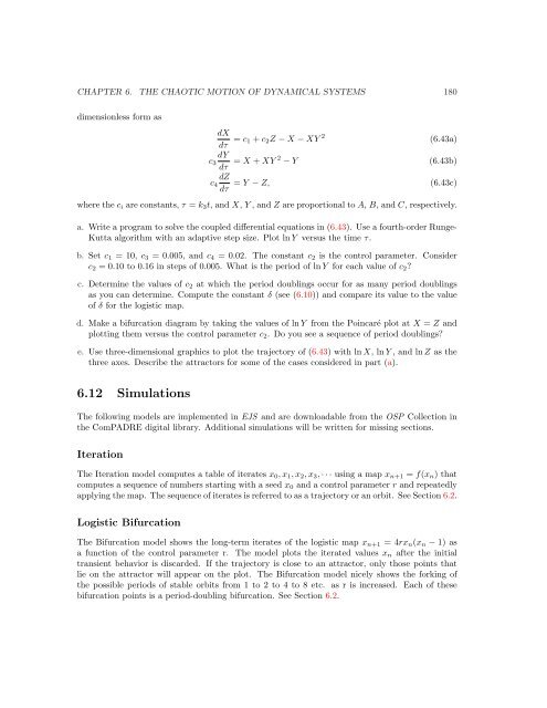
CHAPTER 6. THE CHAOTIC MOTION OF DYNAMICAL SYSTEMS 180dimensionless form asdXdτ = c 1 + c 2 Z − X − XY 2c 3dYdτ = X + XY 2 − Yc 4dZdτ = Y − Z,(6.43a)(6.43b)(6.43c)where the c i are constants, τ = k 3 t, and X, Y , and Z are proportional to A, B, and C, respectively.a. Write a program to solve the coupled differential equations in (6.43). Use a fourth-order Runge-Kutta algorithm with an adaptive step size. Plot ln Y versus the time τ.b. Set c 1 = 10, c 3 = 0.005, and c 4 = 0.02. The constant c 2 is the control parameter. Considerc 2 = 0.10 to 0.16 in steps of 0.005. What is the period of ln Y for each value of c 2 ?c. Determine the values of c 2 at which the period doublings occur for as many period doublingsas you can determine. Compute the constant δ (see (6.10)) and compare its value to the valueof δ for the logistic map.d. Make a bifurcation diagram by taking the values of ln Y from the Poincaré plot at X = Z andplotting them versus the control parameter c 2 . Do you see a sequence of period doublings?e. Use three-dimensional graphics to plot the trajectory of (6.43) with ln X, ln Y , and ln Z as thethree axes. Describe the attractors for some of the cases considered in part (a).6.12 SimulationsThe following models are implemented in EJS and are downloadable from the OSP Collection inthe ComPADRE digital library. Additional simulations will be written for missing sections.IterationThe Iteration model computes a table of iterates x 0 , x 1 , x 2 , x 3 , · · · using a map x n+1 = f(x n ) thatcomputes a sequence of numbers starting with a seed x 0 and a control parameter r and repeatedlyapplying the map. The sequence of iterates is referred to as a trajectory or an orbit. See Section 6.2.Logistic BifurcationThe Bifurcation model shows the long-term iterates of the logistic map x n+1 = 4rx n (x n − 1) asa function of the control parameter r. The model plots the iterated values x n after the initialtransient behavior is discarded. If the trajectory is close to an attractor, only those points thatlie on the attractor will appear on the plot. The Bifurcation model nicely shows the forking ofthe possible periods of stable orbits from 1 to 2 to 4 to 8 etc. as r is increased. Each of thesebifurcation points is a period-doubling bifurcation. See Section 6.2.