Chapter 6 - Davidson Physics

More documents

Recommendations

Info

CHAPTER 6. THE CHAOTIC MOTION OF DYNAMICAL SYSTEMS 171∗ Problem 6.14. Entropy of the logistic mapa. Write a program to compute S for the logistic map. Divide the interval [0, 1] into bins orsubintervals of width ∆x = 0.01 and determine the relative number of times the trajectory fallsinto each bin. At each value of r in the range 0.7 ≤ r ≤ 1. the map should be iterated for afixed number of steps, for example, n = 1000. Choose ∆x = 0.01. What happens to the entropywhen the trajectory is chaotic?b. Repeat part (a) with n = 10000. For what values of r does the entropy change significantly?Decrease ∆x to 0.001 and repeat. Does this decrease make a difference?c. Plot p i as a function of x for r = 1. For what value(s) of x is the plot a maximum?We also can measure the (generalized) entropy as a function of time. As we will see inProblem 6.15, S(n) for strong chaos increases linearly with n until all the possible states arevisited. However, for weak chaos this behavior is not found. In the latter case we can generalizethe entropy to a q-dependent function defined byS q = 1 − ∑ i pq iq − 1. (6.28)In the limit q → 1, S q → S. The following problem discusses measuring the entropy for the samesystem as in Problem 6.13.∗ Problem 6.15. Entropy of weak and strong chaotic systemsa. Write a program that iterates the map (6.25) and plots S if q = 1 or S q if q ≠ 1 as a functionof n. The input parameters should be q, the number of bins, the number of random seeds ina single bin, and n, the number of iterations. At each iteration compute the entropy. Thenaverage S over the randomly chosen values of the seeds.b. Consider strong chaos at a = 2. Choose q = 1, n = 20, at ∆x ≤ 0.001, and ten times asrandomly chosen seeds per bin. Do you obtain a straight line for S versus n? Does the curveeventually stop growing? If you decrease ∆x, how do your results differ and how are they thesame? Show that S is not a linear function of n if q ≠ 1.c. Repeat part (a) with a = 1.401155189 and various values of q. Simulations with 10 5 binsshow that linear behavior is obtained for q ≈ 0.36, the same value as for the measurements inProblem 6.13.
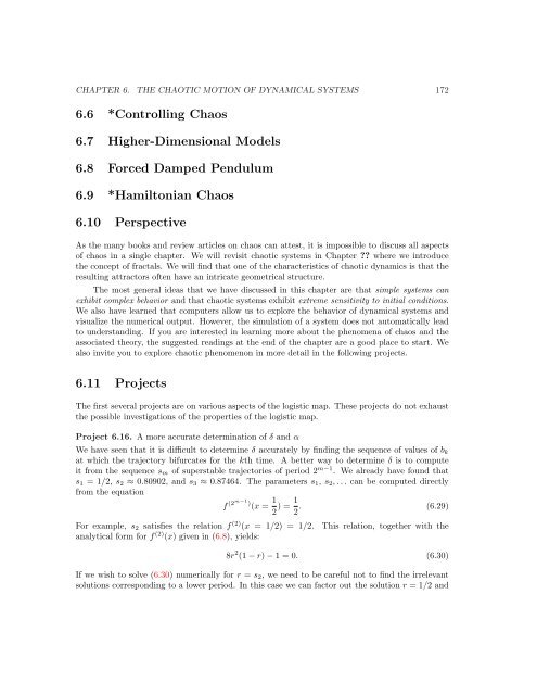
CHAPTER 6. THE CHAOTIC MOTION OF DYNAMICAL SYSTEMS 1726.6 *Controlling Chaos6.7 Higher-Dimensional Models6.8 Forced Damped Pendulum6.9 *Hamiltonian Chaos6.10 PerspectiveAs the many books and review articles on chaos can attest, it is impossible to discuss all aspectsof chaos in a single chapter. We will revisit chaotic systems in <strong>Chapter</strong> ?? where we introducethe concept of fractals. We will find that one of the characteristics of chaotic dynamics is that theresulting attractors often have an intricate geometrical structure.The most general ideas that we have discussed in this chapter are that simple systems canexhibit complex behavior and that chaotic systems exhibit extreme sensitivity to initial conditions.We also have learned that computers allow us to explore the behavior of dynamical systems andvisualize the numerical output. However, the simulation of a system does not automatically leadto understanding. If you are interested in learning more about the phenomena of chaos and theassociated theory, the suggested readings at the end of the chapter are a good place to start. Wealso invite you to explore chaotic phenomenon in more detail in the following projects.6.11 ProjectsThe first several projects are on various aspects of the logistic map. These projects do not exhaustthe possible investigations of the properties of the logistic map.Project 6.16. A more accurate determination of δ and αWe have seen that it is difficult to determine δ accurately by finding the sequence of values of b kat which the trajectory bifurcates for the kth time. A better way to determine δ is to computeit from the sequence s m of superstable trajectories of period 2 m−1 . We already have found thats 1 = 1/2, s 2 ≈ 0.80902, and s 3 ≈ 0.87464. The parameters s 1 , s 2 , . . . can be computed directlyfrom the equationf (2m−1) (x = 1 2 ) = 1 2 . (6.29)For example, s 2 satisfies the relation f (2) (x = 1/2) = 1/2. This relation, together with theanalytical form for f (2) (x) given in (6.8), yields:8r 2 (1 − r) − 1 = 0. (6.30)If we wish to solve (6.30) numerically for r = s 2 , we need to be careful not to find the irrelevantsolutions corresponding to a lower period. In this case we can factor out the solution r = 1/2 and
Page 3 and 4: CHAPTER 6. THE CHAOTIC MOTION OF DY
Page 19: CHAPTER 6. THE CHAOTIC MOTION OF DY
Page 37: CHAPTER 6. THE CHAOTIC MOTION OF DY

Chapter 6 - Davidson Physics

You also want an ePaper? Increase the reach of your titles

Delete template?

Save as template?