Chapter 6 - Davidson Physics

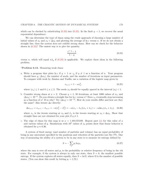
CHAPTER 6. THE CHAOTIC MOTION OF DYNAMICAL SYSTEMS 170which can be checked by substituting (6.23) into (6.22). In the limit q → 1, we recover the usualexponential dependence.We can determine the type of chaos using the crude approach of choosing a large number ofinitial values of x 0 and x 0 + ∆x 0 and plotting the average of ln z versus n. If we do not obtain astraight line, then the system does not exhibit strong chaos. How can we check for the behaviorshown in (6.23)? The easiest way is to plot the quantityz 1−q − 11 − q(6.24)versus n, which will equal nλ q if (6.23) is applicable. We explore these ideas in the followingproblem.∗ Problem 6.13. Measuring weak chaosa. Write a program that plots ln z if q = 1 or z q if q ≠ 1 as a function of n. Your programshould have q, |∆x 0 |, the number of seeds, and the number of iterations as input parameters.To compare with work by Añaños and Tsallis, use a variation of the logistic map given byx n+1 = 1 − ax 2 n, (6.25)where |x n | ≤ 1 and 0 ≤ a ≤ 2. The seeds x 0 should be equally spaced in the interval |x 0 | < 1.b. Consider strong chaos at a = 2. Choose q = 1, 50 iterations, at least 1000 values of x 0 , and|∆x 0 | = 10 −6 . Do you obtain a straight line for ln z versus n? Does z n eventually stop increasingas a function of n? If so why? Try |∆x 0 | = 10 −12 . How do your results differ and how are theythe same? Also iterate ∆x directly:∆x n+1 = x n+1 − ˜x n+1 = −a(x 2 n − ˜x 2 n) = −a(x n − ˜x n )(x n + ˜x n ) = −a∆x n (x n + ˜x n ), (6.26)where x n is the iterate starting at x 0 and ˜x n is the iterate starting at x 0 + ∆x 0 . Show thatstraight lines are not obtained for your plot if q ≠ 1.c. The edge of chaos for this map is at a = 1.401155189. Repeat part (a) for this value of aand various values of q. Simulations with 10 5 values of x 0 points show that linear behavior isobtained for q ≈ 0.36.A system of fixed energy (and number of particles and volume) has an equal probability ofbeing in any microstate specified by the positions and velocities of the particles (see Sec ??). Oneway of measuring the ability of a system to be in any state is to measure its entropy defined byS = − ∑ ip i ln p i , (6.27)where the sum is over all states and p i is the probability or relative frequency of being in the ithstate. For example, if the system is always in only one state, then S = 0, the smallest possibleentropy. If the system explores all states equally, then S = ln Ω, where Ω is the number of possiblestates. (You can show this result by letting p i = 1/Ω.)