Chapter 6 - Davidson Physics

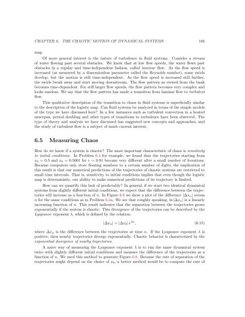
CHAPTER 6. THE CHAOTIC MOTION OF DYNAMICAL SYSTEMS 166map.Of more general interest is the nature of turbulence in fluid systems. Consider a streamof water flowing past several obstacles. We know that at low flow speeds, the water flows pastobstacles in a regular and time-independent fashion, called laminar flow. As the flow speed isincreased (as measured by a dimensionless parameter called the Reynolds number), some swirlsdevelop, but the motion is still time-independent. As the flow speed is increased still further,the swirls break away and start moving downstream. The flow pattern as viewed from the bankbecomes time-dependent. For still larger flow speeds, the flow pattern becomes very complex andlooks random. We say that the flow pattern has made a transition from laminar flow to turbulentflow.This qualitative description of the transition to chaos in fluid systems is superficially similarto the description of the logistic map. Can fluid systems be analyzed in terms of the simple modelsof the type we have discussed here? In a few instances such as turbulent convection in a heatedsaucepan, period doubling and other types of transitions to turbulence have been observed. Thetype of theory and analysis we have discussed has suggested new concepts and approaches, andthe study of turbulent flow is a subject of much current interest.6.5 Measuring ChaosHow do we know if a system is chaotic? The most important characteristic of chaos is sensitivityto initial conditions. In Problem 6.4 for example, we found that the trajectories starting fromx 0 = 0.5 and x 0 = 0.5001 for r = 0.91 become very different after a small number of iterations.Because computers only store floating numbers to a certain number of digits, the implication ofthis result is that our numerical predictions of the trajectories of chaotic systems are restricted tosmall time intervals. That is, sensitivity to initial conditions implies that even though the logisticmap is deterministic, our ability to make numerical predictions of its trajectory is limited.How can we quantify this lack of predictably? In general, if we start two identical dynamicalsystems from slightly different initial conditions, we expect that the difference between the trajectorieswill increase as a function of n. In Figure 6.8 we show a plot of the difference |∆x n | versusn for the same conditions as in Problem 6.4a. We see that roughly speaking, ln |∆x n | is a linearlyincreasing function of n. This result indicates that the separation between the trajectories growsexponentially if the system is chaotic. This divergence of the trajectories can be described by theLyapunov exponent λ, which is defined by the relation:|∆x n | = |∆x 0 | e λn , (6.15)where ∆x n is the difference between the trajectories at time n. If the Lyapunov exponent λ ispositive, then nearby trajectories diverge exponentially. Chaotic behavior is characterized by theexponential divergence of nearby trajectories.A naive way of measuring the Lyapunov exponent λ is to run the same dynamical systemtwice with slightly different initial conditions and measure the difference of the trajectories as afunction of n. We used this method to generate Figure 6.8. Because the rate of separation of thetrajectories might depend on the choice of x 0 , a better method would be to compute the rate of