Chapter 6 - Davidson Physics

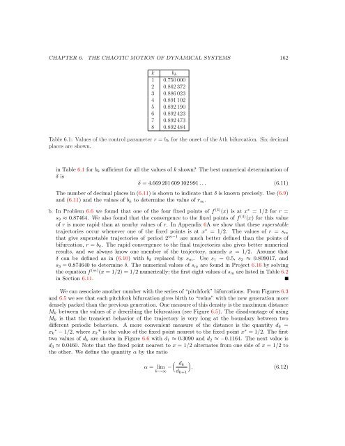
CHAPTER 6. THE CHAOTIC MOTION OF DYNAMICAL SYSTEMS 162k b k1 0.750 0002 0.862 3723 0.886 0234 0.891 1025 0.892 1906 0.892 4237 0.892 4738 0.892 484Table 6.1: Values of the control parameter r = b k for the onset of the kth bifurcation. Six decimalplaces are shown.in Table 6.1 for b k sufficient for all the values of k shown? The best numerical determination ofδ isδ = 4.669 201 609 102 991 . . . (6.11)The number of decimal places in (6.11) is shown to indicate that δ is known precisely. Use (6.9)and (6.11) and the values of b k to determine the value of r ∞ .b. In Problem 6.6 we found that one of the four fixed points of f (4) (x) is at x ∗ = 1/2 for r =s 3 ≈ 0.87464. We also found that the convergence to the fixed points of f (4) (x) for this valueof r is more rapid than at nearby values of r. In Appendix 6A we show that these superstabletrajectories occur whenever one of the fixed points is at x ∗ = 1/2. The values of r = s mthat give superstable trajectories of period 2 m−1 are much better defined than the points ofbifurcation, r = b k . The rapid convergence to the final trajectories also gives better numericalresults, and we always know one member of the trajectory, namely x = 1/2. Assume thatδ can be defined as in (6.10) with b k replaced by s m . Use s 1 = 0.5, s 2 ≈ 0.809017, ands 3 = 0.874640 to determine δ. The numerical values of s m are found in Project 6.16 by solvingthe equation f (m) (x = 1/2) = 1/2 numerically; the first eight values of s m are listed in Table 6.2in Section 6.11.We can associate another number with the series of “pitchfork” bifurcations. From Figures 6.3and 6.5 we see that each pitchfork bifurcation gives birth to “twins” with the new generation moredensely packed than the previous generation. One measure of this density is the maximum distanceM k between the values of x describing the bifurcation (see Figure 6.5). The disadvantage of usingM k is that the transient behavior of the trajectory is very long at the boundary between twodifferent periodic behaviors. A more convenient measure of the distance is the quantity d k =x k ∗ − 1/2, where x k * is the value of the fixed point nearest to the fixed point x ∗ = 1/2. The firsttwo values of d k are shown in Figure 6.6 with d 1 ≈ 0.3090 and d 2 ≈ −0.1164. The next value isd 3 ≈ 0.0460. Note that the fixed point nearest to x = 1/2 alternates from one side of x = 1/2 tothe other. We define the quantity α by the ratio(α = lim − dk). (6.12)k→∞ d k+1