Chapter 6 - Davidson Physics

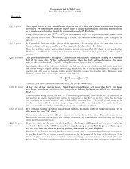
CHAPTER 6. THE CHAOTIC MOTION OF DYNAMICAL SYSTEMS 154The form of f(x) in (6.5) is known as the logistic map. The logistic map is a simple exampleof a dynamical system, that is, the map is a deterministic, mathematical prescription for findingthe future state of a system given its present state.The sequence of values x 0 , x 1 , x 2 , . . . is called the trajectory. To check your understanding,suppose that the initial value of x 0 or seed is x 0 = 0.5 and r = 0.2. Do a calculation to showthat the trajectory is x 1 = 0.2, x 2 = 0.128, x 3 = 0.089293, . . . The first thirty iterations of (6.5) areshown for two values of r in Figure 6.1.1.01.00.80.8xn0.60.4xn0.60.40.20.20.00 10 20 30n(a)0.00 10 20 30n(b)Figure 6.1: (a) The trajectory of x for r = 0.2 and x 0 = 0.6. The stable fixed point is at x = 0.(b) The trajectory for r = 0.7 and x 0 = 0.1. Note the initial transient behavior.The Iterate model in this chapter’s source code directory computes a table of values using amap such as (6.2) or (6.5).Exercise 6.1. IterationAn iterative method for calculating the square root x of a number a is based on the observationthat x = a/x. If we guess the value of the root x and our guess is too small (large), then a/x willbe too large (small) and the average (x + a/x)/2 will be closer to the true value. The true valueof √ a can therefore be found by iteratingx n+1 = (x n + a/x n )/2. (6.6)Use the Iterate model to compute the square root of some representative numbers. Does thealgorithm always converge regardless of the initial guess x 0 ? What happens if a is negative?Problem 6.2. The trajectory of the logistic mapa. Modify the Iterate model to produce a plot of the trajectory to reproduce the results shown inFigure 6.1.b. Use your modified model to explore the dynamical behavior of the logistic map in (6.5) withr = 0.24 for different values of x 0 . Show numerically that x = 0 is a stable fixed point for thisvalue of r. That is, the iterated values of x converge to x = 0 independently of the value of x 0 .If x represents the population of insects, describe the qualitative behavior of the population.

CHAPTER 6. THE CHAOTIC MOTION OF DYNAMICAL SYSTEMS 155c. Explore the dynamical behavior of (6.5) for r = 0.26, 0.5, 0.74, and 0.748. A fixed point isunstable if for almost all values of x 0 near the fixed point, the trajectories diverge from it.Verify that x = 0 is an unstable fixed point for r > 0.25. Show that for the suggested valuesof r, the iterated values of x do not change after an initial transient, that is, the long timedynamical behavior is period 1. In Appendix 6A we show that for r < 3/4 and for x 0 in theinterval 0 < x 0 < 1, the trajectories approach the stable attractor at x = 1 − 1/4r. The set ofinitial points that iterate to the attractor is called the basin of the attractor. For the logisticmap, the interval 0 < x < 1 is the basin of attraction of the attractor x = 1 − 1/4r.d. Explore the dynamical properties of (6.5) for r = 0.752, 0.76, 0.8, and 0.862. For r = 0.752 and0.862 approximately 1000 iterations are necessary to obtain convergent results. Show that if ris greater than 0.75, x oscillates between two values after an initial transient behavior. That is,instead of a stable cycle of period 1 corresponding to one fixed point, the system has a stablecycle of period 2. The value of r at which the single fixed point x ∗ splits or bifurcates into twovalues x 1 ∗ and x 2 ∗ is r = b 1 = 3/4. The pair of x values, x 1 ∗ and x 2 ∗ , form a stable attractorof period 2.e. What are the stable attractors of (6.5) for r = 0.863 and 0.88? What is the correspondingperiod? What are the stable attractors and corresponding periods for r = 0.89, 0.891, and0.8922?A more elegant and useful way to determine the behavior of (6.5) is to plot the long-termvalues of x as a function of r (see Figure 6.2). The Logistic Bifurcation model in this chapter’ssource directory plots the iterated values of x after the initial transient behavior is discarded. Sucha plot is called a bifurcation diagram and is generated by Bifurcate model. For each value of r, thefirst nTransient values of x are computed but not plotted. Then the next nPlot values of x areplotted, with the first half in one color and the second half in another. This process is repeatedfor a new value of r during every evolution step until the desired range of r values is reached. Themagnitude of nPlot should be at least as large as the longest period that you wish to observe.Problem 6.3. Qualitative features of the logistic mapa. Use the Logistic Bifurcation model to identify period 2, period 4, and period 8 behavior as canbe seen in Figure 6.2. Choose nTransient ≥ 1000. It might be necessary to “zoom in” on aportion of the plot. How many period doublings can you find?b. Change the scale so that you can follow the iterations of x from period 4 to period 16 behavior.How does the plot look on this scale in comparison to the original scale?c. Describe the shape of the trajectory near the bifurcations from period 2 to period 4, period 4to 8, etc. These bifurcations are frequently called pitchfork bifurcations.The bifurcation diagram in Figure 6.2 indicates that the period doubling behavior ends atr ≈ 0.892. This value of r is known very precisely and is given by r = r ∞ = 0.892486417967 . . .At r = r ∞ , the sequence of period doublings accumulate to a trajectory of infinite period. InProblem 6.4 we explore the behavior of the trajectories for r > r ∞ .Problem 6.4. Chaotic behavior

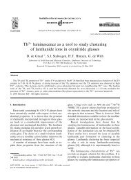
CHAPTER 6. THE CHAOTIC MOTION OF DYNAMICAL SYSTEMS 1561.0iterated values of x0.50.00.7 0.8 0.9r1.0Figure 6.2: Bifurcation diagram of the logistic map. For each value of r, the iterated values ofx n are plotted after the first 1000 iterations are discarded. Note the transition from periodic tochaotic behavior and the narrow windows of periodic behavior within the region of chaos.a. For r > r ∞ , two initial conditions that are very close to one another can yield very differenttrajectories after a few iterations. As an example, choose r = 0.91 and consider x 0 = 0.5 and0.5001. How many iterations are necessary for the iterated values of x to differ by more thanten percent? What happens for r = 0.88 for the same choice of seeds?b. The accuracy of floating point numbers retained on a digital computer is finite. To test theeffect of the finite accuracy of your computer, choose r = 0.91 and x 0 = 0.5 and computethe trajectory for 200 iterations. Then modify your program so that after each iteration, theoperation x = x/10 is followed by x = 10*x. This combination of operations truncates the lastdigit that your computer retains. Compute the trajectory again and compare your results. Doyou find the same discrepancy for r < r ∞ ?c. What are the dynamical properties for r = 0.958? Can you find other windows of periodicbehavior in the interval r ∞ < r < 1?6.3 Period DoublingThe results of the numerical experiments that we did in Section 6.2 probably have convinced youthat the dynamical properties of a simple nonlinear deterministic system can be quite complicated.

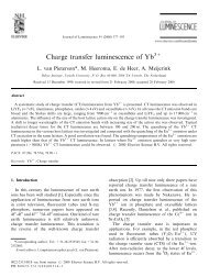
CHAPTER 6. THE CHAOTIC MOTION OF DYNAMICAL SYSTEMS 157To gain more insight into how the dynamical behavior depends on r, we introduce a simplegraphical method for iterating (6.5). In Figure 6.3 we show a graph of f(x) versus x for r = 0.7. Adiagonal line corresponding to y = x intersects the curve y = f(x) at the two fixed points x ∗ = 0and x ∗ = 9/14 ≈ 0.642857 (see (6.7b)). If x 0 is not a fixed point, we can find the trajectory inthe following way. Draw a vertical line from (x = x 0 , y = 0) to the intersection with the curvey = f(x) at (x 0 , y 0 = f(x 0 )). Next draw a horizontal line from (x 0 , y 0 ) to the intersection with thediagonal line at (y 0 , y 0 ). On this diagonal line y = x, and hence the value of x at this intersectionis the first iteration x 1 = y 0 . The second iteration x 2 can be found in the same way. From thepoint (x 1 , y 0 ), draw a vertical line to the intersection with the curve y = f(x). Keep y fixed aty = y 1 = f(x 1 ), and draw a horizontal line until it intersects the diagonal line; the value of x atthis intersection is x 2 . Further iterations can be found by repeating this process.1.0y0.50.00.0 0.5x1.0Figure 6.3: Graphical representation of the iteration of the logistic map (6.5) with r = 0.7 andx 0 = 0.9. Note that the graphical solution converges to the fixed point x ∗ ≈ 0.643.This graphical method is illustrated in Figure 6.3 for r = 0.7 and x 0 = 0.9. If we begin withany x 0 (except x 0 = 0 and x 0 = 1), the iterations will converge to the fixed point x ∗ ≈ 0.643. Itwould be a good idea to repeat the procedure shown in Figure 6.3 by hand. For r = 0.7, the fixedpoint is stable (an attractor of period 1). In contrast, no matter how close x 0 is to the fixed pointat x = 0, the iterates diverge away from it, and this fixed point is unstable.How can we explain the qualitative difference between the fixed point at x = 0 and at x ∗ =0.642857 for r = 0.7? The local slope of the curve y = f(x) determines the distance movedhorizontally each time f is iterated. A slope steeper than 45 ◦ leads to a value of x further awayfrom its initial value. Hence, the criterion for the stability of a fixed point is that the magnitude

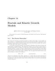
CHAPTER 6. THE CHAOTIC MOTION OF DYNAMICAL SYSTEMS 158of the slope at the fixed point must be less than 45 ◦ . That is, if |df(x)/dx| x=x ∗ is less than unity,then x ∗ is stable; conversely, if |df(x)/dx| x=x ∗ is greater than unity, then x ∗ is unstable.An inspection of f(x) in Figure 6.3 shows that x = 0 is unstable because the slope of f(x) atx = 0 is greater than unity. In contrast, the magnitude of the slope of f(x) at x = x ∗ ≈ 0.643 isless than unity and this fixed point is stable. In Appendix 6A, we show thatandx ∗ = 0 is stable for 0 < r < 1/4,x ∗ = 1 − 1 4ris stable for 1/4 < r < 3/4.(6.7b)(6.7a)Thus for 0 < r < 3/4, the behavior after many iterations is known.What happens if r is greater than 3/4? We found in Section 6.2 that if r is slightly greaterthan 3/4, the fixed point of f becomes unstable and bifurcates to a cycle of period 2. Now xreturns to the same value after every second iteration, and the fixed points of f ( f(x) ) are thestable attractors of f(x). In the following, we write f (2) (x) = f ( f(x) ) and f (n) (x) for the nthiterate of f(x). (Do not confuse f (n) (x) with the nth derivative of f(x).) For example, the seconditerate f (2) (x) is given by the fourth-order polynomial:f (2) (x) = 4r [ 4rx(1 − x) ] − 4r [ 4rx(1 − x) ] 2= 4r[4rx(1 − x)] [ 1 − 4rx(1 − x) ]= 16r 2 x [ − 4rx 3 + 8rx 2 − (1 + 4r)x + 1 ] . (6.8)What happens if we increase r still further? Eventually the magnitude of the slope of the fixedpoints of f (2) (x) exceeds unity and the fixed points of f (2) (x) become unstable. Now the cycle off is period 4, and the fixed points of the fourth iterate f (4) (x) = f (2)( f (2) (x) ) = f ( f ( f(f(x) ))are stable. These fixed points also eventually become unstable, and we are led to the phenomenaof period doubling that we observed in Problem 6.3.The Logistic Cobweb model in the chapter’s code directory implements the graphical analysisof the iterations of f(x). The nth order iterates are defined using the recursive methodf(x,iterate) shown in Listing 6.1. (The parameter iterate is 1, 2, and 4 for the functions f(x),f (2) (x), and f (4) (x) respectively and the value of the control parameter is 0.8.) Recursion is anidea that is simple once you understand it, but it can be difficult to grasp initially. Although themethod calls itself, the rules for method calls remain the same. Imagine that a recursive methodis called. The computer then starts to execute the code in the method, but comes to another callof the same method as itself. At this point the computer stops executing the code of the originalmethod, and makes an exact copy of the method with possibly different input parameters, andstarts executing the code in the copy. There are now two possibilities. One is that the computercomes to the end of the copy without another recursive call. In that case the computer deletes thecopy of the method and continues executing the code in the original method. The other possibilityis that a recursive call is made in the copy, and a third copy is made of the method, and the code inthe third copy is now executed. This process continues until the code in all the copies is executed.Every recursive method must have a possibility of reaching the end of the method; otherwise, theprogram will eventually crash.

CHAPTER 6. THE CHAOTIC MOTION OF DYNAMICAL SYSTEMS 159f(1)f(1)f(2)f(2)f(2)f(2)f(3)f(3)f(3)f(3)f(3)f(3)answer(a) (b) (c) (d) (e) (f)Figure 6.4: Example of the calculation of f(0.4,3) using the recursive function defined in theLogistic Cobweb model. The number in each box is the value of the variable iterate. Thecomputer executes code from left to right, and each box represents a copy of the function in thecomputer’s memory. The input values x = 0.4 and r = 0.8, which are the same in each copy, arenot shown. The arrows indicate when a copy is finished and its value is returned to one of theother copies. Notice that the first copy of the function, f(3), is the last one to finish. The value off(x,3) = 0.7842.Listing 6.1: The f(x,iterate) custom method evaluates the logistic function recursively.public double f ( double x , int i t e r a t e ) {x=4*r*x*(1−x ) ; // compute new xi f ( i t e r a t e ==1) return x ;else return f ( x , i t e r a t e −1);}To understand the method f(x,iterate), suppose we want to compute f(0.4,3). First wewrite f(0.4,3) as in Figure 6.4a. Follow the statements within the method until another call tof(0.4,iterate) occurs. In this case, the call is to f(0.4,iterate-1) which equals f(0.4,2).Write f(0.4,2) above f(0.4,3) (see Figure 6.4b). When you come to the end of the definition ofthe method, write down the value of f that is actually returned, and remove the method from thestack by crossing it out (see Figure 6.4d). This returned value for f equals y if iterate > 1, orit is the value of the logistic function for iterate = 1. Continue deleting copies of f as they arefinished, until there are no copies left on the paper. The final value of f is the value returned bythe computer.Exercise 6.5. RecursionCreate a simple model that defines the control parameter r and the f(x,iterate) custommethod and prints the value of the input parameters x and iterate when the method is invoked.Test your method with f(0.4,3). Is the answer the same as your hand calculation?Problem 6.6. Qualitative properties of the fixed pointsa. Use the Logistic Cobweb model to show graphically that there is a single stable fixed point off(x) for r < 3/4. It would be instructive to modify the program so that the value of the slope

CHAPTER 6. THE CHAOTIC MOTION OF DYNAMICAL SYSTEMS 160df/dx| x=xn is shown as you step each iteration. At what value of r does the absolute value ofthis slope exceed unity? Let b 1 denote the value of r at which the fixed point of f(x) bifurcatesand becomes unstable. Verify that b 1 = 0.75.b. Describe the trajectory of f(x) for r = 0.785. Is the fixed point given by x = 1 − 1/4r stableor unstable? What is the nature of the trajectory if x 0 = 1 − 1/4r? What is the period of f(x)for all other choices of x 0 ? What are the values of the two-point attractor?c. The function f(x) is symmetrical about x = 1/2 where f(x) is a maximum. What are thequalitative features of the second iterate f (2) (x) for r = 0.785? Is f (2) (x) symmetrical aboutx = 1/2? For what value of x does f (2) (x) have a minimum? Iterate x n+1 = f (2) (x n ) forr = 0.785 and find its two fixed points x 1 ∗ and x 2 ∗ . (Try x 0 = 0.1 and x 0 = 0.3.) Are the fixedpoints of f (2) (x) stable or unstable for this value of r? How do these values of x 1 ∗ and x 2∗compare with the values of the two-point attractor of f(x)? Verify that the slopes of f (2) (x) atx 1 ∗ and x 2 ∗ are equal.d. Verify the following properties of the fixed points of f (2) (x). As r is increased, the fixed pointsof f (2) (x) move apart and the slope of f (2) (x) at its fixed points decreases. What is the valueof r = s 2 at which one of the two fixed points of f (2) equals 1/2? What is the value of theother fixed point? What is the slope of f (2) (x) at x = 1/2? What is the slope at the otherfixed point? As r is further increased, the slopes at the fixed points become negative. Finallyat r = b 2 ≈ 0.8623, the slopes at the two fixed points of f (2) (x) equal −1, and the two fixedpoints of f (2) become unstable. (The exact value of b 2 is b 2 = (1 + √ 6)/4.)e. Show that for r slightly greater than b 2 , for example, r = 0.87, there are four stable fixed pointsof f (4) (x). What is the value of r = s 3 when one of the fixed points equals 1/2? What are thevalues of the three other fixed points at r = s 3 ?f. Determine the value of r = b 3 at which the four fixed points of f (4) become unstable.g. Choose r = s 3 and determine the number of iterations that are necessary for the trajectory toconverge to period 4 behavior. How does this number of iterations change when neighboringvalues of r are considered? Choose several values of x 0 so that your results do not depend onthe initial conditions.Problem 6.7. Periodic windows in the chaotic regimea. If you look closely at the bifurcation diagram in Figure 6.2, you will see that the range ofchaotic behavior for r > r ∞ is interrupted by intervals of periodic behavior. Magnify yourbifurcation diagram so that you can look at the interval 0.957107 ≤ r ≤ 0.960375, where aperiodic trajectory of period 3 occurs. (Period 3 behavior starts at r = (1 + √ 8)/4.) Whathappens to the trajectory for slightly larger r, for example, r = 0.9604?b. Plot f (3) (x) versus x at r = 0.96, a value of r in the period 3 window. Draw the line y = xand determine the intersections with f (3) (x). The stable fixed points satisfy the condition x ∗ =f (3) (x ∗ ). Because f (3) (x) is an eighth-order polynomial, there are eight solutions (including x =0). Find the intersections of f (3) (x) with y = x and identify the three stable fixed points. Whatare the slopes of f (3) (x) at these points? Then decrease r to r = 0.957107, the (approximate)

CHAPTER 6. THE CHAOTIC MOTION OF DYNAMICAL SYSTEMS 161value of r below which the system is chaotic. Draw the line y = x and determine the number ofintersections with f (3) (x). Note that at this value of r, the curve y = f (3) (x) is tangent to thediagonal line at the three stable fixed points. For this reason, this type of transition is called atangent bifurcation. Note that there also is an unstable point at x ≈ 0.76.c. Plot x n+1 = f (3) (x n ) versus n for r = 0.9571, a value of r just below the onset of period 3behavior. How would you describe the behavior of the trajectory? This type of chaotic motion isan example of intermittency, that is, nearly periodic behavior interrupted by occasional irregularbursts.d. To understand the mechanism for the intermittent behavior, we need to “zoom in” on the valuesof x near the stable fixed points that you found in part (c). To do so change the scale of theplot. You will see a narrow channel between the diagonal line y = x and the plot of f (3) (x) neareach fixed point. The trajectory can require many iterations to squeeze through the channel,and we see apparent period 3 behavior during this time. Eventually, the trajectory escapes fromthe channel and bounces around until it is again enters a channel at some unpredictable latertime.6.4 Universal Properties and Self-SimilarityIn Sections 6.2 and 6.12 we found that the trajectory of the logistic map has remarkable propertiesas a function of the control parameter r. In particular, we found a sequence of period doublingsaccumulating in a chaotic trajectory of infinite period at r = r ∞ . For most values of r > r ∞ ,the trajectory is very sensitive to the initial conditions. We also found “windows” of period 3, 6,12, . . . embedded in the range of chaotic behavior. How typical is this type of behavior? In thefollowing, we will find further numerical evidence that the general behavior of the logistic map isindependent of the details of the form (6.5) of f(x).You might have noticed that the range of r between successive bifurcations becomes smalleras the period increases (see Table 6.1). For example, b 2 − b 1 = 0.112398, b 3 − b 2 = 0.023624, andb 4 − b 3 = 0.00508. A good guess is that the decrease in b k − b k−1 is geometric, that is, the ratio(b k − b k−1 )/(b k+1 − b k ) is a constant. You can check that this ratio is not exactly constant, butconverges to a constant with increasing k. This behavior suggests that the sequence of values ofb k has a limit and follows a geometrical progression:b k ≈ r ∞ − C δ −k , (6.9)where δ is known as the Feigenbaum number and C os a constant. From (6.9) it is easy to showthat δ is given by the ratiob k − b k−1δ = lim . (6.10)k→∞ b k+1 − b kProblem 6.8. Estimation of the Feigenbaum constanta. Derive the relation (6.10) given (6.9). Plot δ k = (b k − b k−1 )/(b k+1 − b k ) versus k using thevalues of b k in Table 6.1 and determine the value of δ. Are the number of decimal places given

CHAPTER 6. THE CHAOTIC MOTION OF DYNAMICAL SYSTEMS 162k b k1 0.750 0002 0.862 3723 0.886 0234 0.891 1025 0.892 1906 0.892 4237 0.892 4738 0.892 484Table 6.1: Values of the control parameter r = b k for the onset of the kth bifurcation. Six decimalplaces are shown.in Table 6.1 for b k sufficient for all the values of k shown? The best numerical determination ofδ isδ = 4.669 201 609 102 991 . . . (6.11)The number of decimal places in (6.11) is shown to indicate that δ is known precisely. Use (6.9)and (6.11) and the values of b k to determine the value of r ∞ .b. In Problem 6.6 we found that one of the four fixed points of f (4) (x) is at x ∗ = 1/2 for r =s 3 ≈ 0.87464. We also found that the convergence to the fixed points of f (4) (x) for this valueof r is more rapid than at nearby values of r. In Appendix 6A we show that these superstabletrajectories occur whenever one of the fixed points is at x ∗ = 1/2. The values of r = s mthat give superstable trajectories of period 2 m−1 are much better defined than the points ofbifurcation, r = b k . The rapid convergence to the final trajectories also gives better numericalresults, and we always know one member of the trajectory, namely x = 1/2. Assume thatδ can be defined as in (6.10) with b k replaced by s m . Use s 1 = 0.5, s 2 ≈ 0.809017, ands 3 = 0.874640 to determine δ. The numerical values of s m are found in Project 6.16 by solvingthe equation f (m) (x = 1/2) = 1/2 numerically; the first eight values of s m are listed in Table 6.2in Section 6.11.We can associate another number with the series of “pitchfork” bifurcations. From Figures 6.3and 6.5 we see that each pitchfork bifurcation gives birth to “twins” with the new generation moredensely packed than the previous generation. One measure of this density is the maximum distanceM k between the values of x describing the bifurcation (see Figure 6.5). The disadvantage of usingM k is that the transient behavior of the trajectory is very long at the boundary between twodifferent periodic behaviors. A more convenient measure of the distance is the quantity d k =x k ∗ − 1/2, where x k * is the value of the fixed point nearest to the fixed point x ∗ = 1/2. The firsttwo values of d k are shown in Figure 6.6 with d 1 ≈ 0.3090 and d 2 ≈ −0.1164. The next value isd 3 ≈ 0.0460. Note that the fixed point nearest to x = 1/2 alternates from one side of x = 1/2 tothe other. We define the quantity α by the ratio(α = lim − dk). (6.12)k→∞ d k+1

CHAPTER 6. THE CHAOTIC MOTION OF DYNAMICAL SYSTEMS 163y0.90.7M 1M 20.50.30.7 0.8r0.9Figure 6.5: The first few bifurcations of the logistic equation showing the scaling of the maximumdistance M k between the asymptotic values of x describing the bifurcation.The ratios α = (0.3090/0.1164) = 2.65 for k = 1 and α = (0.1164/0.0460) = 2.53 for k = 2 areconsistent with the asymptotic value α = 2.5029078750958928485 . . .We now give qualitative arguments that suggest that the general behavior of the logistic mapin the period doubling regime is independent of the detailed form of f(x). As we have seen, perioddoubling is characterized by self-similarities, for example, the period doublings look similar exceptfor a change of scale. We can demonstrate these similarities by comparing f(x) for r = s 1 = 0.5for the superstable trajectory with period 1 to the function f (2) (x) for r = s 2 ≈ 0.809017 for thesuperstable trajectory of period 2 (see Figure 6.7). The function f(x, r = s 1 ) has unstable fixedpoints at x = 0 and x = 1 and a stable fixed point at x = 1/2. Similarly the function f (2) (x, r = s 2 )has a stable fixed point at x = 1/2 and an unstable fixed point at x ≈ 0.69098. Note the similarshape, but different scale of the curves in the square boxes in part (a) and part (b) of Figure 6.7.This similarity is an example of scaling. That is, if we scale f (2) and change (renormalize) the valueof r, we can compare f (2) to f. (See Chapter ?? for a discussion of scaling and renormalization inanother context.)This graphical comparison is meant only to be suggestive. A precise approach shows that ifwe continue the comparison of the higher-order iterates, for example, f (4) (x) to f (2) (x), etc., thesuperposition of functions converges to a universal function that is independent of the form of theoriginal function f(x).Problem 6.9. Further determinations of the exponents α and δ

CHAPTER 6. THE CHAOTIC MOTION OF DYNAMICAL SYSTEMS 164y0.90.7d 1d 20.50.30.7 0.8r0.9Figure 6.6: The quantity d k is the distance from x ∗ = 1/2 to the nearest element of the attractorof period 2 k . It is convenient to use this quantity to determine the exponent α.1. Determine the appropriate scaling factor and superimpose f and the rescaled form of f (2)found in Figure 6.7.2. Use arguments similar to those discussed in the text and in Figure 6.7 and compare thebehavior of f (4) (x, r = s 3 ) in the square about x = 1/2 with f (2) (x, r = s 2 ) in its squareabout x = 1/2. The size of the squares are determined by the unstable fixed point nearestto x = 1/2. Find the appropriate scaling factor and superimpose f (2) and the rescaled formof f (4) .∗ Problem 6.10. Other one-dimensional mapsIt is easy to modify your programs to consider other one-dimensional maps. Determine the qualitativeproperties of the one-dimensional maps:f(x) = xe r(1−x) (6.13)f(x) = r sin πx. (6.14)Do they also exhibit the period doubling route to chaos? The map in (6.13) has been used byecologists (cf. May) to study a population that is limited at high densities by the effect of epidemics.Although it is more complicated than (6.5), its advantage is that the population remains positive

CHAPTER 6. THE CHAOTIC MOTION OF DYNAMICAL SYSTEMS 1651.01.0f(x)f (2) (x)0.50.50.00.5 1.0x0.00.5 1.0x(a)(b)Figure 6.7: Comparison of f(x, r) for r = s 1 with the second iterate f (2) (x) for r = s 2 . (a) Thefunction f(x, r = s 1 ) has unstable fixed points at x = 0 and x = 1 and a stable fixed point atx = 1/2. (b) The function f (2) (x, r = s 1 ) has a stable fixed point at x = 1/2. The unstable fixedpoint of f (2) (x) nearest to x = 1/2 occurs at x ≈ 0.69098, where the curve f (2) (x) intersects theline y = x. The upper right-hand corner of the square box in (b) is located at this point, and thecenter of the box is at (1/2, 1/2). Note that if we reflect this square about the point (1/2, 1/2),the shape of the reflected graph in the square box is nearly the same as it is in part (a), but on asmaller scale.no matter what (positive) value is taken for the initial population. There are no restrictions onthe maximum value of r, but if r becomes sufficiently large, x eventually becomes effectively zero.What is the behavior of the time series of (6.13) for r = 1.5, 2, and 2.7? Describe the qualitativebehavior of f(x). Does it have a maximum?The sine map (6.14) with 0 < r ≤ 1 and 0 ≤ x ≤ 1 has no special significance, except that itis nonlinear. If time permits, determine the approximate value of δ for both maps. What limitsthe accuracy of your determination of δ?The above qualitative arguments and numerical results suggest that the quantities α and δ areuniversal, that is, independent of the detailed form of f(x). In contrast, the values of the accumulationpoint r ∞ and the constant C in (6.9) depend on the detailed form of f(x). Feigenbaum hasshown that the period doubling route to chaos and the values of δ and α are universal propertiesof maps that have a quadratic maximum, that is, f ′ (x) |x=xm = 0 and f ′′ (x) |x=xm < 0.Why is the universality of period doubling and the numbers δ and α more than a curiosity?The reason is that because this behavior is independent of the details, there might exist realisticsystems whose underlying dynamics yield the same behavior as the logistic map. Of course, mostphysical systems are described by differential rather than difference equations. Can these systemsexhibit period doubling behavior? Several workers (cf. Testa et al.) have constructed nonlinearRLC circuits driven by an oscillatory source voltage. The output voltage shows bifurcations, andthe measured values of the exponents δ and α are consistent with the predictions of the logistic

CHAPTER 6. THE CHAOTIC MOTION OF DYNAMICAL SYSTEMS 166map.Of more general interest is the nature of turbulence in fluid systems. Consider a streamof water flowing past several obstacles. We know that at low flow speeds, the water flows pastobstacles in a regular and time-independent fashion, called laminar flow. As the flow speed isincreased (as measured by a dimensionless parameter called the Reynolds number), some swirlsdevelop, but the motion is still time-independent. As the flow speed is increased still further,the swirls break away and start moving downstream. The flow pattern as viewed from the bankbecomes time-dependent. For still larger flow speeds, the flow pattern becomes very complex andlooks random. We say that the flow pattern has made a transition from laminar flow to turbulentflow.This qualitative description of the transition to chaos in fluid systems is superficially similarto the description of the logistic map. Can fluid systems be analyzed in terms of the simple modelsof the type we have discussed here? In a few instances such as turbulent convection in a heatedsaucepan, period doubling and other types of transitions to turbulence have been observed. Thetype of theory and analysis we have discussed has suggested new concepts and approaches, andthe study of turbulent flow is a subject of much current interest.6.5 Measuring ChaosHow do we know if a system is chaotic? The most important characteristic of chaos is sensitivityto initial conditions. In Problem 6.4 for example, we found that the trajectories starting fromx 0 = 0.5 and x 0 = 0.5001 for r = 0.91 become very different after a small number of iterations.Because computers only store floating numbers to a certain number of digits, the implication ofthis result is that our numerical predictions of the trajectories of chaotic systems are restricted tosmall time intervals. That is, sensitivity to initial conditions implies that even though the logisticmap is deterministic, our ability to make numerical predictions of its trajectory is limited.How can we quantify this lack of predictably? In general, if we start two identical dynamicalsystems from slightly different initial conditions, we expect that the difference between the trajectorieswill increase as a function of n. In Figure 6.8 we show a plot of the difference |∆x n | versusn for the same conditions as in Problem 6.4a. We see that roughly speaking, ln |∆x n | is a linearlyincreasing function of n. This result indicates that the separation between the trajectories growsexponentially if the system is chaotic. This divergence of the trajectories can be described by theLyapunov exponent λ, which is defined by the relation:|∆x n | = |∆x 0 | e λn , (6.15)where ∆x n is the difference between the trajectories at time n. If the Lyapunov exponent λ ispositive, then nearby trajectories diverge exponentially. Chaotic behavior is characterized by theexponential divergence of nearby trajectories.A naive way of measuring the Lyapunov exponent λ is to run the same dynamical systemtwice with slightly different initial conditions and measure the difference of the trajectories as afunction of n. We used this method to generate Figure 6.8. Because the rate of separation of thetrajectories might depend on the choice of x 0 , a better method would be to compute the rate of

CHAPTER 6. THE CHAOTIC MOTION OF DYNAMICAL SYSTEMS 16710 -2|∆x n |10 -410 -610 -80 10 20 30 40 50nFigure 6.8: The evolution of the difference ∆x n between the trajectories of the logistic map atr = 0.91 for x 0 = 0.5 and x 0 = 0.5001. The separation between the two trajectories increases withn, the number of iterations, if n is not too large. (Note that |∆x 1 | ∼ 10 −8 and that the trend isnot monotonic.)separation for many values of x 0 . This method would be tedious, because we would have to fit theseparation to (6.15) for each value of x 0 and then determine an average value of λ.A more important limitation of the naive method is that because the trajectory is restrictedto the unit interval, the separation |∆x n | ceases to increase when n becomes sufficiently large.Fortunately, there is a better way of determining λ. We take the natural logarithm of both sidesof (6.15), and write λ asλ = 1 n ln ∣ ∣∣∣ ∆x n∆x 0∣ ∣∣∣. (6.16)Because we want to use the data from the entire trajectory after the transient behavior has ended,we use the fact that∆x n= ∆x 1 ∆x 2 ∆x n· · · . (6.17)∆x 0 ∆x 0 ∆x 1 ∆x n−1Hence, we can express λ asλ = 1 n−1∑∣ ln∆x i+1 ∣∣∣n ∣ . (6.18)∆x iThe form (6.18) implies that we can interpret x i for any i as the initial condition.i=0We see from (6.18) that the problem of computing λ has been reduced to finding the ratio∆x i+1 /∆x i . Because we want to make the initial difference between the two trajectories as smallas possible, we are interested in the limit ∆x i → 0.

CHAPTER 6. THE CHAOTIC MOTION OF DYNAMICAL SYSTEMS 1681.0λ0.0-1.0-2.00.7 0.8 0.9 1.0rFigure 6.9: The Lyapunov exponent calculated using the method in (6.20) as a function of thecontrol parameter r. Compare the behavior of λ to the bifurcation diagram in Figure 6.2. Notethat λ < 0 for r < 3/4 and approaches zero at a period doubling bifurcation. A negative spikecorresponds to a superstable trajectory. The onset of chaos is visible near r = 0.892, where λfirst becomes positive. For r 0.892, λ generally increases except for dips below zero whenevera periodic window occurs, for example, the dip due to the period 3 window near r = 0.96. Foreach value of r, the first 1000 iterations were discarded, and 10 5 values of ln |f ′ (x n )| were used todetermine λ.The idea of the more sophisticated procedure is to compute dx i+1 /dx i from the equation ofmotion at the same time that the equation of motion is being iterated. We use the logistic map asan example. From (6.5) we havedx i+1dx i= f ′ (x i ) = 4r(1 − 2x i ). (6.19)We can consider x i for any i as the initial condition and the ratio dx i+1 /dx i as a measure of therate of change of x i . Hence, we can iterate the logistic map as before and use the values of x i andthe relation (6.19) to compute f ′ (x i ) = dx i+1 /dx i at each iteration. The Lyapunov exponent isgiven byn−11 ∑λ = lim ln |f ′ (x i )| , (6.20)n→∞ ni=0where we begin the sum in (6.20) after the transient behavior is finished. We have includedexplicitly the limit n → ∞ in (6.20) to remind ourselves to choose n sufficiently large. Note that

CHAPTER 6. THE CHAOTIC MOTION OF DYNAMICAL SYSTEMS 169this procedure weights the points on the attractor correctly, that is, if a particular region of theattractor is not visited often by the trajectory, it does not contribute much to the sum in (6.20).Exercise 6.11. Nearby trajectoriesCreate model to reproduce Figure 6.8 and compute the Lyapunov exponent λ using the naiveapproach. Choose r = 0.91, x 0 = 0.5, and ∆x 0 = 10 −6 , and plot ln |∆x n /∆x 0 | versus n. Whathappens to ln |∆x n /∆x 0 | for large n? Determine λ for r = 0.91, r = 0.97, and r = 1.0. Does yourresult for λ for each value of r depend significantly on your choice of x 0 or ∆x 0 ?Problem 6.12. Lyapunov exponent for the logistic mapa. Use the Logistic Lyapunov model to study λ using the algorithm discussed in the text forr = 0.76 to r = 1.0 in steps of ∆r = 0.01. What is the sign of λ if the system is not chaotic?Plot λ versus r, and explain your results in terms of behavior of the bifurcation diagram shownin Figure 6.2. Compare your results for λ with those shown in Figure 6.9. How does the sign ofλ correlate with the behavior of the system as seen in the bifurcation diagram? For what valueof r is λ a maximum?b. In Problem 6.4b we saw that roundoff errors in the chaotic regime make the computation ofindividual trajectories meaningless. That is, if the system’s behavior is chaotic, then smallroundoff errors are amplified exponentially in time, and the actual numbers we compute for thetrajectory starting from a given initial value are not “real.” Repeat your calculation of λ forr = 1 by changing the roundoff error as you did in Problem 6.4b. Does your computed value ofλ change? How meaningful is your computation of the Lyapunov exponent? We will encountera similar question in Chapter 8 where we compute the trajectories of chaotic systems of manyparticles. We will find that although the “true” trajectories cannot be computed for long times,averages over the trajectories yield meaningful results.We have found that nearby trajectories diverge if λ > 0. For λ < 0, the two trajectoriesconverge and the system is not chaotic. What happens for λ = 0? In this case we will see thatthe trajectories diverge algebraically, that is, as a power of n. In some cases a dynamical systemis at the “edge of chaos” where the Lyapunov exponent vanishes. Such systems are said to exhibitweak chaos to distinguish their behavior from the strongly chaotic behavior (λ > 0) that we havebeen discussing.If we define z ≡ |∆x n |/|∆x 0 |, then z will satisfy the differential equationdz= λz. (6.21)dnFor weak chaos we do not find an exponential divergence, but instead a divergence that is algebraicand is given bydzdn = λ qz q , (6.22)where q is a parameter that needs to be determined. The solution to (6.22) isz = [1 + (1 − q)λ q n] 1/(1−q) , (6.23)

CHAPTER 6. THE CHAOTIC MOTION OF DYNAMICAL SYSTEMS 170which can be checked by substituting (6.23) into (6.22). In the limit q → 1, we recover the usualexponential dependence.We can determine the type of chaos using the crude approach of choosing a large number ofinitial values of x 0 and x 0 + ∆x 0 and plotting the average of ln z versus n. If we do not obtain astraight line, then the system does not exhibit strong chaos. How can we check for the behaviorshown in (6.23)? The easiest way is to plot the quantityz 1−q − 11 − q(6.24)versus n, which will equal nλ q if (6.23) is applicable. We explore these ideas in the followingproblem.∗ Problem 6.13. Measuring weak chaosa. Write a program that plots ln z if q = 1 or z q if q ≠ 1 as a function of n. Your programshould have q, |∆x 0 |, the number of seeds, and the number of iterations as input parameters.To compare with work by Añaños and Tsallis, use a variation of the logistic map given byx n+1 = 1 − ax 2 n, (6.25)where |x n | ≤ 1 and 0 ≤ a ≤ 2. The seeds x 0 should be equally spaced in the interval |x 0 | < 1.b. Consider strong chaos at a = 2. Choose q = 1, 50 iterations, at least 1000 values of x 0 , and|∆x 0 | = 10 −6 . Do you obtain a straight line for ln z versus n? Does z n eventually stop increasingas a function of n? If so why? Try |∆x 0 | = 10 −12 . How do your results differ and how are theythe same? Also iterate ∆x directly:∆x n+1 = x n+1 − ˜x n+1 = −a(x 2 n − ˜x 2 n) = −a(x n − ˜x n )(x n + ˜x n ) = −a∆x n (x n + ˜x n ), (6.26)where x n is the iterate starting at x 0 and ˜x n is the iterate starting at x 0 + ∆x 0 . Show thatstraight lines are not obtained for your plot if q ≠ 1.c. The edge of chaos for this map is at a = 1.401155189. Repeat part (a) for this value of aand various values of q. Simulations with 10 5 values of x 0 points show that linear behavior isobtained for q ≈ 0.36.A system of fixed energy (and number of particles and volume) has an equal probability ofbeing in any microstate specified by the positions and velocities of the particles (see Sec ??). Oneway of measuring the ability of a system to be in any state is to measure its entropy defined byS = − ∑ ip i ln p i , (6.27)where the sum is over all states and p i is the probability or relative frequency of being in the ithstate. For example, if the system is always in only one state, then S = 0, the smallest possibleentropy. If the system explores all states equally, then S = ln Ω, where Ω is the number of possiblestates. (You can show this result by letting p i = 1/Ω.)

CHAPTER 6. THE CHAOTIC MOTION OF DYNAMICAL SYSTEMS 171∗ Problem 6.14. Entropy of the logistic mapa. Write a program to compute S for the logistic map. Divide the interval [0, 1] into bins orsubintervals of width ∆x = 0.01 and determine the relative number of times the trajectory fallsinto each bin. At each value of r in the range 0.7 ≤ r ≤ 1. the map should be iterated for afixed number of steps, for example, n = 1000. Choose ∆x = 0.01. What happens to the entropywhen the trajectory is chaotic?b. Repeat part (a) with n = 10000. For what values of r does the entropy change significantly?Decrease ∆x to 0.001 and repeat. Does this decrease make a difference?c. Plot p i as a function of x for r = 1. For what value(s) of x is the plot a maximum?We also can measure the (generalized) entropy as a function of time. As we will see inProblem 6.15, S(n) for strong chaos increases linearly with n until all the possible states arevisited. However, for weak chaos this behavior is not found. In the latter case we can generalizethe entropy to a q-dependent function defined byS q = 1 − ∑ i pq iq − 1. (6.28)In the limit q → 1, S q → S. The following problem discusses measuring the entropy for the samesystem as in Problem 6.13.∗ Problem 6.15. Entropy of weak and strong chaotic systemsa. Write a program that iterates the map (6.25) and plots S if q = 1 or S q if q ≠ 1 as a functionof n. The input parameters should be q, the number of bins, the number of random seeds ina single bin, and n, the number of iterations. At each iteration compute the entropy. Thenaverage S over the randomly chosen values of the seeds.b. Consider strong chaos at a = 2. Choose q = 1, n = 20, at ∆x ≤ 0.001, and ten times asrandomly chosen seeds per bin. Do you obtain a straight line for S versus n? Does the curveeventually stop growing? If you decrease ∆x, how do your results differ and how are they thesame? Show that S is not a linear function of n if q ≠ 1.c. Repeat part (a) with a = 1.401155189 and various values of q. Simulations with 10 5 binsshow that linear behavior is obtained for q ≈ 0.36, the same value as for the measurements inProblem 6.13.

CHAPTER 6. THE CHAOTIC MOTION OF DYNAMICAL SYSTEMS 1726.6 *Controlling Chaos6.7 Higher-Dimensional Models6.8 Forced Damped Pendulum6.9 *Hamiltonian Chaos6.10 PerspectiveAs the many books and review articles on chaos can attest, it is impossible to discuss all aspectsof chaos in a single chapter. We will revisit chaotic systems in Chapter ?? where we introducethe concept of fractals. We will find that one of the characteristics of chaotic dynamics is that theresulting attractors often have an intricate geometrical structure.The most general ideas that we have discussed in this chapter are that simple systems canexhibit complex behavior and that chaotic systems exhibit extreme sensitivity to initial conditions.We also have learned that computers allow us to explore the behavior of dynamical systems andvisualize the numerical output. However, the simulation of a system does not automatically leadto understanding. If you are interested in learning more about the phenomena of chaos and theassociated theory, the suggested readings at the end of the chapter are a good place to start. Wealso invite you to explore chaotic phenomenon in more detail in the following projects.6.11 ProjectsThe first several projects are on various aspects of the logistic map. These projects do not exhaustthe possible investigations of the properties of the logistic map.Project 6.16. A more accurate determination of δ and αWe have seen that it is difficult to determine δ accurately by finding the sequence of values of b kat which the trajectory bifurcates for the kth time. A better way to determine δ is to computeit from the sequence s m of superstable trajectories of period 2 m−1 . We already have found thats 1 = 1/2, s 2 ≈ 0.80902, and s 3 ≈ 0.87464. The parameters s 1 , s 2 , . . . can be computed directlyfrom the equationf (2m−1) (x = 1 2 ) = 1 2 . (6.29)For example, s 2 satisfies the relation f (2) (x = 1/2) = 1/2. This relation, together with theanalytical form for f (2) (x) given in (6.8), yields:8r 2 (1 − r) − 1 = 0. (6.30)If we wish to solve (6.30) numerically for r = s 2 , we need to be careful not to find the irrelevantsolutions corresponding to a lower period. In this case we can factor out the solution r = 1/2 and

CHAPTER 6. THE CHAOTIC MOTION OF DYNAMICAL SYSTEMS 173m period s m1 1 0.500 000 0002 2 0.809 016 9943 4 0.874 640 4254 8 0.888 660 9705 16 0.891 666 8996 32 0.892 310 8837 64 0.892 448 8238 128 0.892 478 091Table 6.2: Values of the control parameter s m for the superstable trajectories of period 2 m−1 . Ninedecimal places are shown.solve the resultant quadratic equation analytically to find s 2 = (1 + √ 5)/4. Clearly r = s 1 = 1/2solves (6.30) with period 1, because from (6.29), f (1) (x = 1/2) = 4r 1 2 (1 − 1 2) = r = 1/2 only forr = 1/2.1. It is straightforward to adapt the bisection method discussed in Section 6.6. Adapt theclass RecursiveFixedPointApp to find the numerical solutions of (6.29). Good startingvalues for the left-most and right-most values of r are easy to obtain. The left-most value isr = r ∞ ≈ 0.8925. If we already know the sequence s 1 , s 2 , . . . , s m , then we can determine δbyδ m = s m−1 − s m−2. (6.31)s m − s m−1We use this determination for δ m to find the right-most value of r:r (m+1)right= s m − s m−1δ m. (6.32)We choose the desired precision to be 10 −16 . A summary of our results is given in Table 6.2.Verify these results and determine δ.2. Use your values of s m to obtain a more accurate determination of α and δ.Project 6.17. From chaos to orderThe bifurcation diagram of the logistic map (see Figure 6.2) has many interesting features thatwe have not explored. For example, you might have noticed that there are several smooth darkbands in the chaotic region for r > r ∞ . Use BifurcateApp to generate the bifurcation diagram forr ∞ ≤ r ≤ 1. If we start at r = 1.0 and decrease r, we see that there is a band that narrows andeventually splits into two parts at r ≈ 0.9196. If you look closely, you will see that the band splitsinto four parts at r ≈ 0.899. If you look even more closely, you will see many more bands. Whattype of change occurs near the splitting (merging) of these bands)? Use IterateMap to look atthe time series of (6.5) for r = 0.9175. You will notice that although the trajectory looks random,it oscillates back and forth between two bands. This behavior can be seen more clearly if you lookat the time series of x n+1 = f (2) (x n ). A detailed discussion of the splitting of the bands can befound in Peitgen et al.

CHAPTER 6. THE CHAOTIC MOTION OF DYNAMICAL SYSTEMS 174Project 6.18. Calculation of the Lyapunov spectrumIn Section 6.12 we discussed the calculation of the Lyapunov exponent for the logistic map. If adynamical system has a multidimensional phase space, for example, the Hénon map and the Lorenzmodel, there is a set of Lyapunov exponents, called the Lyapunov spectrum, that characterize thedivergence of the trajectory. As an example, consider a set of initial conditions that forms a filledsphere in phase space for the (three-dimensional) Lorenz model. If we iterate the Lorenz equations,then the set of phase space points will deform into another shape. If the system has a fixed point,this shape contracts to a single point. If the system is chaotic, then, typically, the sphere willdiverge in one direction, but become smaller in the other two directions. In this case we can definethree Lyapunov exponents to measure the deformation in three mutually perpendicular directions.These three directions generally will not correspond to the axes of the original variables. Instead,we must use a Gram-Schmidt orthogonalization procedure.The algorithm for finding the Lyapunov spectrum is as follows:(i) Linearize the dynamical equations. If r is the f-component vector containing the dynamicalvariables, then define ∆r as the linearized difference vector. For example, the linearizedLorenz equations ared∆x= −σ∆x + σ∆ydt(6.33a)d∆y= −x∆z − z∆x + r∆x − ∆ydt(6.33b)d∆z= x∆y + y∆x − b∆z.dt(6.33c)(ii) Define f orthonormal initial values for ∆r. For example, ∆r 1 (0) = (1, 0, 0), ∆r 2 (0) = (0, 1, 0),and ∆r 3 (0) = (0, 0, 1). Because these vectors appear in a linearized equation, they do nothave to be small in magnitude.(iii) Iterate the original and linearized equations of motion. One iteration yields a new vectorfrom the original equation of motion and f new vectors ∆r α from the linearized equations.(iv) Find the orthonormal vectors ∆r ′ α from the ∆r α using the Gram-Schmidt procedure. Thatis,∆r ′ 1 = ∆r 1|∆r 1 |∆r ′ 2 = ∆r 2 − (∆r ′ 1 · ∆r 2 )∆r ′ 1|∆r 2 − (∆r ′ 1 · ∆r 2)∆r ′ 1 |∆r ′ 3 = ∆r 3 − (∆r ′ 1 · ∆r 3 )∆r ′ 1 − (∆r ′ 2 · ∆r 3 )∆r∣′ 2∣∆r 3 − (∆r ′ 1 · ∆r 3)∆r ′ 1 − (∆r′ 2 · ∆r 3)∆r ′ ∣ .2(6.34a)(6.34b)(6.34c)It is straightforward to generalize the method to higher dimensional models.(v) Set the ∆r α (t) equal to the orthonormal vectors ∆r ′ α(t).(vi) Accumulate the running sum, S α as S α → S α + log |∆r α (t)|.

CHAPTER 6. THE CHAOTIC MOTION OF DYNAMICAL SYSTEMS 175(vii) Repeat steps (iii)–(vi) and periodically output the approximate Lyapunov exponents λ α =(1/n)S α , where n is the number of iterations.To obtain a result for the Lyapunov spectrum that represent the steady state attractor, only includedata after the transient behavior has ended.a. Compute the Lyapunov spectrum for the Lorenz model for σ = 16, b = 4, and r = 45.92. Tryother values of the parameters and compare your results.b. Linearize the equations for the Hénon map and find the Lyapunov spectrum for a = 1.4 andb = 0.3 in (??).Project 6.19. A spinning magnetConsider a compass needle that is free to rotate in a periodically reversing magnetic field which isperpendicular to the axis of the needle. The equation of motion of the needle is given byd 2 φdt 2 = −µ I B 0 cos ωt sin φ, (6.35)where φ is the angle of the needle with respect to a fixed axis along the field, µ is the magneticmoment of the needle, I its moment of inertia, and B 0 and ω are the amplitude and theangular frequency of the magnetic field, respectively. Choose an appropriate numerical methodfor solving (6.35), and plot the Poincaré map at time t = 2πn/ω. Verify that if the parameterλ = √ 2B 0 µ/I/ω 2 > 1, then the motion of the needle exhibits chaotic motion. Briggs (seereferences) discusses how to construct the corresponding laboratory system and other nonlinearphysical systems.LLrr(a)(b)Figure 6.10: (a) Geometry of the stadium billiard model. (b) Geometry of the Sinai billiard model.Project 6.20. Billiard modelsConsider a two-dimensional planar geometry in which a particle moves with constant velocity alongstraight line orbits until it elastically reflects off the boundary. This straight line motion occurs invarious “billiard” systems. A simple example of such a system is a particle moving with fixed speed

CHAPTER 6. THE CHAOTIC MOTION OF DYNAMICAL SYSTEMS 176within a circle. For this geometry the angle between the particle’s momentum and the tangent tothe boundary at a reflection is the same for all points.Suppose that we divide the circle into two equal parts and connect them by straight lines oflength L as shown in Figure 6.10a. This geometry is called a stadium billiard. How does the motionof a particle in the stadium compare to the motion in the circle? In both cases we can find thetrajectory of the particle by geometrical considerations. The stadium billiard model and a similargeometry known as the Sinai billiard model (see Figure 6.10b) have been used as model systemsfor exploring the foundations of statistical mechanics. There also is much interest in relating thebehavior of a classical particle in various billiard models to the solution of Schrödinger’s equationfor the same geometries.a. Write a program to simulate the stadium billiard model. Use the radius r of the semicircles asthe unit of length. The algorithm for determining the path of the particle is as follows:(i) Begin with an initial position (x 0 , y 0 ) and momentum (p x0 , p y0 ) of the particle such that|p 0 | = 1.(ii) Determine which of the four sides the particle will hit. The possibilities are the top andbottom line segments and the right and left semicircles.(iii) Determine the next position of the particle from the intersection of the straight line definedby the current position and momentum, and the equation for the segment where the nextreflection occurs.(iv) Determine the new momentum, (p ′ x, p ′ y), of the particle after reflection such that the angleof incidence equals the angle of reflection. For reflection off the line segments we have(p ′ x, p ′ y) = (p x , −p y ). For reflection off a circle we havep ′ x = [ y 2 − (x − x c ) 2] p x − 2(x − x c )yp yp ′ y = −2(x − x c )yp x + [ (x − x c ) 2 − y 2] p y ,(6.36a)(6.36b)where (x c , 0) is the center of the circle. (Note that the momentum p x rather than p ′ x is onthe right-hand side of (6.36b). Remember that all lengths are scaled by the radius of thecircle.)(v) Repeat steps (ii)–(iv).b. Determine if the particle dynamics is chaotic by estimating the largest Lyapunov exponent. Oneway to do so is to start two particles with almost identical positions and/or momenta (varyingby say 10 −5 ). Compute the difference ∆s of the two phase space trajectories as a function ofthe number of reflections n, where ∆s is defined by∆s = √ |r 1 − r 2 | 2 + |p 1 − p 2 | 2 . (6.37)Choose L = 1 and r = 1. The Lyapunov exponent can be found from a semilog plot of ∆sversus n. Repeat your calculation for different initial conditions and average your values of ∆sbefore plotting. Repeat the calculation for L = 0.5 and 2.0 and determine if your results dependon L.

CHAPTER 6. THE CHAOTIC MOTION OF DYNAMICAL SYSTEMS 177c. Another test for the existence of chaos is the reversibility of the motion. Reverse the momentumafter the particle has made n reflections, and let the drawing color equal the background colorso that the path can be erased. What limitation does roundoff error place on your results?Repeat this simulation for L = 1 and L = 0.d. Place a small hole of diameter d in one of the circular sections of the stadium so that theparticle can escape. Choose L = 1 and set d = 0.02. Give the particle a random position andmomentum, and record the time when the particle escapes through the hole. Repeat for atleast 10 4 particles and compute the fraction of particles S(n) remaining after a given numberof reflections n. The function S(n) will decay with n. Determine the functional dependence ofS on n, and calculate the characteristic decay time if S(n) decays exponentially. Repeat forL = 0.1, 0.5, and 2.0. Is the decay time a function of L? Does S(n) decays exponentially forthe circular billiard model (L = 0) (see Bauer and Bertsch)?e. Choose an arbitrary initial position for the particle in a stadium with L = 1, and a small hole asin part (d). Choose at least 5000 values of the initial value p x0 uniformly distributed between0 and 1. Choose p y0 so that |p| = 1. Plot the escape time versus p x0 , and describe the visualpattern of the trajectories. Then choose 5000 values of p x0 in a smaller interval centered aboutthe value of p x0 for which the escape time was greatest. Plot these values of the escape timeversus p x0 . Do you see any evidence of self-similarity?f. Repeat steps (a)–(e) for the Sinai billiard geometry.Project 6.21. The circle map and mode lockingThe driven, damped pendulum can be approximated by a one-dimensional difference equation fora range of amplitudes and frequencies of the driving force. This difference equation is known asthe circle map and is given byθ n+1 =(θ n + Ω − K )2π sin 2πθ n . (modulo 1) (6.38)The variable θ represents an angle, and Ω represents a frequency ratio, the ratio of the naturalfrequency of the pendulum to the frequency of the periodic driving force. The parameter K isa measure of the strength of the nonlinear coupling of the pendulum to the external force. Animportant quantity is the winding number which is defined aswhere ∆θ n = Ω − (K/2π) sin 2πθ n .m−11 ∑W = lim ∆θ n , (6.39)m→∞ ma. Consider the linear case, K = 0. Choose Ω = 0.4 and θ 0 = 0.2 and determine W . Verify thatif Ω is a ratio of two integers, then W = Ω and the trajectory is periodic. What is the valueof W if Ω = √ 2/2, an irrational number? Verify that W = Ω and that the trajectory comesarbitrarily close to any particular value of θ. Does θ n ever return exactly to its initial value?This type of behavior of the trajectory is termed quasiperiodic.n=0

CHAPTER 6. THE CHAOTIC MOTION OF DYNAMICAL SYSTEMS 178b. For K > 0, we will find that W ≠ Ω and “locks” into rational frequency ratios for a range ofvalues of K and Ω. This type of behavior is called mode locking. For K < 1, the trajectory iseither periodic or quasiperiodic. Determine the value of W for K = 1/2 and values of Ω in therange O < Ω ≤ 1. The widths in Ω of the various mode-locked regions where W is fixed increasewith K. Consider other values of K, and draw a diagram in the K-Ω plane (0 ≤ K, Ω ≤ 1)so that those areas corresponding to frequency locking are shaded. These shaded regions arecalled Arnold tongues.c. For K = 1, all trajectories are frequency-locked periodic trajectories. Fix K at K = 1 anddetermine the dependence of W on Ω. The plot of W versus Ω for K = 1 is called the Devil’sstaircase.Project 6.22. Chaotic scatteringIn Chapter 5 we discussed the classical scattering of particles off a fixed target, and found thatthe differential cross section for a variety of interactions is a smoothly varying function of thescattering angle. That is, a small change in the impact parameter b leads to a small change in thescattering angle θ. Here we consider examples where a small change in b leads to large changes inθ. Such a phenomenon is called chaotic scattering, because of the sensitivity to initial conditionsthat is characteristic of chaos. The study of chaotic scattering is relevant to the design of electronicnanostructures, because many experimental structures exhibit this type of scattering.A typical scattering model consists of a target composed of a group of fixed hard disks anda scatterer consisting of a point particle. The goal is to compute the path of the scatterer as itbounces off the disks, and measure θ and the time of flight as a function of the impact parameterb. If a particle bounces inside the target region before leaving, the time of flight can be very long.There are even some trajectories for which the particle never leaves the target region.Because it is difficult to monitor a trajectory that bounces back and forth between the harddisks, we instead consider a two-dimensional map that contains the key features of chaotic scattering(see Yalcinkaya and Lai for further discussion). The map is given byx n+1 = a [ x n − 1 4 (x n + y n ) 2] ,(6.40a)y n+1 = 1 a[yn + 1 4 (x n + y n ) 2] , (6.40b)where a is a parameter. The target region is centered at the origin. In an actual scatteringexperiment, the relation between (x n+1 , y n+1 ) and (x n , y n ) would be much more complicated, butthe map (6.40) captures most of the important features of realistic chaotic scattering experiments.The iteration number n is analogous to the number of collisions of the scattered particle off thedisks. When x n or y n is significantly different from zero, the scatterer has left the target region.a. Write a program to iterate the map (6.40). Let a = 8.0 and y 0 = −0.3. Choose 10 4 initial valuesof x 0 uniformly distributed in the interval 0 < x 0 < 0.1. Determine the time T (x 0 ), the numberof iterations for which x n ≤ −5.0. After this time, x n rapidly moves to −∞. Plot T (x 0 ) versusx 0 . Then choose 10 4 initial values in a smaller interval centered about a value of x 0 for whichT (x 0 ) > 7. Plot these values of T (x 0 ) versus x 0 . Do you see any evidence of self-similarity?

CHAPTER 6. THE CHAOTIC MOTION OF DYNAMICAL SYSTEMS 179b. A trajectory is said to be uncertain if a small change ɛ in x 0 leads to a change in T (x 0 ). Weexpect that the number of uncertain trajectories, N, will depend on a power of ɛ, that is,N ∼ ɛ α . Determine N(ɛ) for ɛ = 10 −p with p = 2 to 7 using the values of x 0 in part (a). Thendetermine the uncertainty dimension 1 − α from a log-log plot of N versus ɛ. Repeat thesemeasurements for other values of a. Does α depend on a?c. Choose 4×10 4 initial conditions in the same interval as in part (a) and determine the number oftrajectories, S(n), that have not yet reached x n = −5 as a function of the number of iterationsn. Plot ln S(n) versus n and determine if the decay is exponential. It is possible to obtainalgebraic decay for values of a less than approximately 6.5.d. Let a = 4.1 and choose 100 initial conditions uniformly distributed in the region 1.0 < x 0 < 1.05and 0.60 < y 0 < 0.65. Are there any trajectories that are periodic and hence have infinite escapetimes? Due to the accumulation of roundoff error, it is possible to find only finite, but very longescape times. These periodic trajectories form closed curves, and the regions enclosed by themare called KAM surfaces.Project 6.23. Chemical reactionsIn Project 4.20 we discussed how chemical oscillations can occur when the reactants are continuouslyreplenished. In this project we introduce a set of chemical reactions that exhibits the perioddoubling route to chaos. Consider the following reactions (see Peng et al.):P → AP + C → A + CA → BA + 2B → 3BB → CC → D.(6.41a)(6.41b)(6.41c)(6.41d)(6.41e)(6.41f)Each of the above reactions has an associated rate constant. The time dependence of the concentrationsof A, B, and C is given by:dAdt = k 1P + k 2 P C − k 3 A − k 4 AB 2dBdt = k 3A + k 4 AB 2 − k 5 BdCdt = k 4B − k 5 C.(6.42a)(6.42b)(6.42c)We assume that P is held constant by replenishment from an external source. We also assumethe chemicals are well mixed so that there is no spatial dependence. In Section ?? we discuss theeffects of spatial inhomogeneities due to molecular diffusion. Equations (6.41) can be written in a

CHAPTER 6. THE CHAOTIC MOTION OF DYNAMICAL SYSTEMS 180dimensionless form asdXdτ = c 1 + c 2 Z − X − XY 2c 3dYdτ = X + XY 2 − Yc 4dZdτ = Y − Z,(6.43a)(6.43b)(6.43c)where the c i are constants, τ = k 3 t, and X, Y , and Z are proportional to A, B, and C, respectively.a. Write a program to solve the coupled differential equations in (6.43). Use a fourth-order Runge-Kutta algorithm with an adaptive step size. Plot ln Y versus the time τ.b. Set c 1 = 10, c 3 = 0.005, and c 4 = 0.02. The constant c 2 is the control parameter. Considerc 2 = 0.10 to 0.16 in steps of 0.005. What is the period of ln Y for each value of c 2 ?c. Determine the values of c 2 at which the period doublings occur for as many period doublingsas you can determine. Compute the constant δ (see (6.10)) and compare its value to the valueof δ for the logistic map.d. Make a bifurcation diagram by taking the values of ln Y from the Poincaré plot at X = Z andplotting them versus the control parameter c 2 . Do you see a sequence of period doublings?e. Use three-dimensional graphics to plot the trajectory of (6.43) with ln X, ln Y , and ln Z as thethree axes. Describe the attractors for some of the cases considered in part (a).6.12 SimulationsThe following models are implemented in EJS and are downloadable from the OSP Collection inthe ComPADRE digital library. Additional simulations will be written for missing sections.IterationThe Iteration model computes a table of iterates x 0 , x 1 , x 2 , x 3 , · · · using a map x n+1 = f(x n ) thatcomputes a sequence of numbers starting with a seed x 0 and a control parameter r and repeatedlyapplying the map. The sequence of iterates is referred to as a trajectory or an orbit. See Section 6.2.Logistic BifurcationThe Bifurcation model shows the long-term iterates of the logistic map x n+1 = 4rx n (x n − 1) asa function of the control parameter r. The model plots the iterated values x n after the initialtransient behavior is discarded. If the trajectory is close to an attractor, only those points thatlie on the attractor will appear on the plot. The Bifurcation model nicely shows the forking ofthe possible periods of stable orbits from 1 to 2 to 4 to 8 etc. as r is increased. Each of thesebifurcation points is a period-doubling bifurcation. See Section 6.2.

CHAPTER 6. THE CHAOTIC MOTION OF DYNAMICAL SYSTEMS 181Logistic CobwebThe Logistic Cobweb model shows the behavior of the logistic map by showing a cobweb plot, atable of iterates, and a plot of iterates. The cobweb plot consists of a diagonal (x = y) line and acurve representing y = 4rx(1 − x). Starting with an initial seed x 0 , the plot shows how visuallyhow the logistic map produces successive iterates. The cobweb spirals inward toward a stable fixedpoint. Period doubling produces closed loops, and chaotic orbits show a filled area. See Section .Logistic LyapunovThe Logistic Lyapunov Exponent model plots the Lyapunov exponent to shows the rate of separationof logistic map trajectories. See Section .Two Ball BounceThe Two Ball Bounce model shows a two-ball collision in a constant gravitational field that isconstrained to move in one dimension above a fixed floor. Except when a collision occurs, eachball is a freely falling particle. The model also displays a Poincaré map using the velocity v 1 andheight y 1 of the upper ball m1 at the instant that the lower ball m 2 hits the floor.Appendix 6A: Stability of the Fixed Points of the LogisticMapIn the following, we derive analytical expressions for the fixed points of the logistic map. Thefixed-point condition is given byx ∗ = f(x ∗ ). (6.44)From (6.5) this condition yields the two fixed pointsx ∗ = 0 and x ∗ = 1 − 1 4r . (6.45)Because x is restricted to be positive, the only fixed point for r < 1/4 is x = 0. To determine thestability of x ∗ , we letandBecause |ɛ n | ≪ 1, we havex n = x ∗ + ɛ n ,x n+1 = x ∗ + ɛ n+1 .(6.46a)(6.46b)x n+1 = f(x ∗ + ɛ n ) ≈ f(x ∗ ) + ɛ n f ′ (x ∗ ) = x ∗ + ɛ n f ′ (x ∗ ). (6.47)If we compare (6.46b) and (6.47), we obtainɛ n+1 /ɛ n = f ′ (x ∗ ). (6.48)

CHAPTER 6. THE CHAOTIC MOTION OF DYNAMICAL SYSTEMS 182If |f ′ (x ∗ )| > 1, the trajectory will diverge from x ∗ because |ɛ n+1 | > |ɛ n |. The opposite istrue for |f ′ (x ∗ )| < 1. Hence, the local stability criteria for a fixed point x ∗ are1. |f ′ (x ∗ )| < 1, x ∗ is stable;2. |f ′ (x ∗ )| = 1, x ∗ is marginally stable;3. |f ′ (x ∗ )| > 1, x ∗ is unstable.If x ∗ is marginally stable, the second derivative f ′′ (x) must be considered, and the trajectoryapproaches x ∗ with deviations from x ∗ inversely proportional to the square root of the number ofiterations.For the logistic map the derivatives at the fixed points are respectivelyandf ′ (x = 0) = ddx [4rx(1 − x)] ∣∣∣∣x=0= 4r, (6.49)f ′ (x = x ∗ ) = ddx [4rx(1 − x)] ∣∣∣∣x=1−1/4r= 2 − 4r. (6.50)It is straightforward to use (6.49) and (6.50) to find the range of r for which x ∗ = 0 and x ∗ = 1−1/4rare stable.If a trajectory has period two, then f (2) (x) = f(f(x)) has two fixed points. If you areinterested, you can solve for these fixed points analytically. As we found in Problem 6.3, thesetwo fixed points become unstable at the same value of r. We can derive this property of the fixedpoints using the chain rule of differentiation:ddx f (2) (x) ∣ x=x0= ddx f(f(x))∣ ∣x=x0= f ′ (f(x 0 ))f ′ (x) ∣ x=x0. (6.51)If we substitute x 1 = f(x 0 ), we can writeIn the same way, we can show thatddx f(f(x))∣ ∣x=x0= f ′ (x 1 )f ′ (x 0 ). (6.52)ddx f (2) (x) ∣ ∣x=x1= f ′ (x 0 )f ′ (x 1 ). (6.53)We see that if x 0 becomes unstable, then |f (2)′ (x 0 )| > 1 as does |f (2)′ (x 1 )|. Hence, x 1 also isunstable at the same value of r, and we conclude that both fixed points of f (2) (x) bifurcate at thesame value of r, leading to an trajectory of period 4.From (6.50) we see that f ′ (x = x ∗ ) = 0 when r = 1/2 and x ∗ = 1/2. Such a fixed point is saidto be superstable, because as we found in Problem 6.6, convergence to the fixed point is relativelyrapid. Superstable trajectories occur whenever one of the fixed points is at x ∗ = 1/2.

CHAPTER 6. THE CHAOTIC MOTION OF DYNAMICAL SYSTEMS 183Appendix 6B: Finding the Roots of a FunctionThe roots of a function f(x) are the values of the variable x for which the function f(x) is zero.Even an apparently simple equation such aswhere c is a constant cannot be solved analytically for x.f(x) = tan x − x − c = 0. (6.54)Regardless of the function and the approach to root finding, the first step should be to learn asmuch as possible about the function. For example, plotting the function will help us to determinethe approximate locations of the roots.Newton’s (or the Newton-Raphson) method is based on replacing the function by the firsttwo terms of the Taylor expansion of f(x) about the root x. If our initial guess for the root isx 0 , we can write f(x) ≈ f(x 0 ) + (x − x 0 )f ′ (x 0 ). If we set f(x) equal to zero and solve for x, wefind x = x 0 − f(x 0 )/f ′ (x 0 ). If we have made a good choice for x 0 , the resultant value of x shouldbe closer than x 0 to the root. The general procedure is to calculate successive approximations asfollows:x n+1 = x n − f(x n)f ′ (x n ) . (6.55)If this series converges, it converges very quickly. However, if the initial guess is poor or if thefunction has closely spaced multiple roots, the series may not converge. The successive iterationsof Newton’s method is an another example of a map. Newton’s method also works with complexfunctions as we will see in the following problem.Problem 6.24. Cube rootsConsider the function f(z) = z 3 − 1, where z = x + iy, and f ′ (z) = z 2 . Map the range ofconvergence of (6.55) in the region [−2 < x < 2, −2 < y < 2] in the complex plane. Color thestarting z value red, green, or blue depending on the root to which the initial guess converges. Ifthe trajectory does not converge, color the starting point black. For more insight add a mousehandler to your program so that if you click on your plot, the sequence of iterations starting fromthe point where you clicked will be shown.The following problem discusses a situation that typically arises in courses on quantum mechanics.Problem 6.25. Energy levels in a finite square wellThe quantum mechanical energy levels in the one-dimensional finite square well can be found bysolving the relation:ɛ tan ɛ = √ ρ 2 − ɛ 2 , (6.56)where ɛ = √ mEa 2 /2 and ρ = √ mV 0 a 2 /2 are defined in terms of the particle mass m, theparticle energy E, the width of the well a, and the depth of the well V 0 . The function ɛ tan ɛ haszeros at ɛ = 0, π, 2π, . . . and asymptotes at ɛ = 0, π/2, 3π/2, 5π/2 . . .. The function √ ρ − ɛ 2 is aquarter circle of radius ρ. Write a program to plot these two functions with ρ = 3 and then useNewton’s method to determine the roots of (6.56). Find the value of ρ and thus V 0 , such thatbelow this value there is only one energy level and above this value there is more than one. Atwhat value of ρ do three energy levels first appear?

CHAPTER 6. THE CHAOTIC MOTION OF DYNAMICAL SYSTEMS 184In Section 6.6 we introduced the bisection root finding algorithm. This algorithm is implementedin the Root class in the numerics package. It can be used with any function.Listing 6.2: The bisection method defined in the Root class in the numerics package.public s t a t i c double b i s e c t i o n ( f i n a l Function f , double x1 , double x2 , f i n a l double t o l ) {int count = 0 ;int maxCount = ( int ) (Math . l o g (Math . abs ( x2 − x1 ) / t o l ) / Math . l o g ( 2 ) ) ;maxCount = Math . max(MAX ITERATIONS, maxCount ) + 2 ;double y1 = f . e v a l u a t e ( x1 ) , y2 = f . e v a l u a t e ( x2 ) ;i f ( y1 * y2 > 0) { // y1 and y2 must have o p p o s i t e s i g nreturn Double .NaN; // i n t e r v a l does not contain a r o o t}while ( count < maxCount ) {double x = ( x1 + x2 ) / 2 ;double y = f . e v a l u a t e ( x ) ;i f (Math . abs ( y ) < t o l ) return x ;i f ( y * y1 > 0) { // r e p l a c e t h e end−p o i n t t h a t has t h e same s i g nx1 = x ;y1 = y ;}else {x2 = x ;y2 = y ;}count++;}return Double .NaN; // did not converge in max i t e r a t i o n s}The bisection algorithm is guaranteed to converge if you can find an interval where the functionchanges sign. However, it is slow. Newton’s algorithm is very fast, but may not converge. Wedevelop an algorithm in the following problem that combines these two approaches.Problem 6.26. Finding rootsModify Newton’s algorithm to keep track of the interval between the minimum and the maximumof x while iterating (6.55). If the iterate x n+1 jumps outside this interval, interrupt Newton’smethod and use the bisection algorithm for one iteration. Test the root at the end of the iterativeprocess to check that the algorithm actually found a root. Test your algorithm on the function in(6.54).References and Suggestions for Further ReadingBooksRalph H. Abraham and Christopher D. Shaw, Dynamics – The Geometry of Behavior, secondedition, Addison-Wesley (1992). The authors use an abundance of visual representations.

CHAPTER 6. THE CHAOTIC MOTION OF DYNAMICAL SYSTEMS 185Hao Bai-Lin, Chaos II, World Scientific (1990). A collection of reprints on chaotic phenomena.The following papers were cited in the text. James P. Crutchfield, J. Doyne Farmer, NormanH. Packhard, and Robert S. Shaw, “Chaos,” Sci. Am. 255 (6), 46–57 (1986); Mitchell J.Feigenbaum, “Quantitative universality for a class of nonlinear transformations,” J. Stat.Phys. 19, 25–52 (1978); M. Hénon, “A two-dimensional mapping with a strange attractor,”Commun. Math. Phys. 50, 69–77 (1976); Robert M. May, “Simple mathematical models withvery complicated dynamics,” Nature 261, 459–467 (1976); Robert Van Buskirk and CarsonJeffries, “Observation of chaotic dynamics of coupled nonlinear oscillators,” Phys. Rev. A31, 3332–3357 (1985).G. L. Baker and J. P. Gollub, Chaotic Dynamics: An Introduction, second edition, CambridgeUniversity Press (1995). A good introduction to chaos with special emphasis on the forceddamped nonlinear harmonic oscillator. Several programs are given.Pedrag Cvitanovic, Universality in Chaos, second edition, Adam-Hilger (1989). A collection ofreprints on chaotic phenomena including the articles by Hénon and May also reprinted inthe Bai-Lin collection and the chaos classic, Mitchell J. Feigenbaum, “Universal behavior innonlinear systems,” Los Alamos Sci. 1, 4–27 (1980).Robert Devaney, A First Course in Chaotic Dynamical Systems, Addison-Wesley (1992). Thistext is a good introduction to the more mathematical ideas behind chaos and related topics.Jan Fröyland, Introduction to Chaos and Coherence, Institute of Physics Publishing (1992). SeeChapter 7 for a simple model of Saturn’s rings.Martin C. Gutzwiller, Chaos in Classical and Quantum Mechanics, Springer-Verlag (1990). Agood introduction to problems in quantum chaos for the more advanced student.Robert C. Hilborn, Chaos and Nonlinear Dynamics, Oxford University Press (1994). An excellentpedagogically oriented text.Douglas R. Hofstadter, Metamagical Themas, Basic Books (1985). A shorter version is given inhis article, “Metamagical themas,” Sci. Am. 245 (11), 22–43 (1981).E. Atlee Jackson, Perspectives of Nonlinear Dynamics, Vols. 1 and 2., Cambridge University Press(1989, 1991). An advanced text that is a joy to read.R. V. Jensen, “Chaotic scattering, unstable periodic orbits, and fluctuations in quantum transport,”Chaos 1, 101–109 (1991). This paper discusses the quantum version of systems similarto those discussed in Projects 6.22 and 6.20.Francis C. Moon, Chaotic and Fractal Dynamics, An Introduction for Applied Scientists andEngineers, Wiley (1992). An engineering oriented text with a section on how to build devicesthat demonstrate chaotic dynamics.Edward Ott, Chaos in Dynamical Systems, Cambridge University Press (1993). An excellenttextbook on chaos at the upper undergraduate to graduate level. See also E. Ott, “Strangeattractors and chaotic motions of dynamical systems,” Rev. Mod. Phys. 53, 655–671 (1981).

CHAPTER 6. THE CHAOTIC MOTION OF DYNAMICAL SYSTEMS 186Edward Ott, Tim Sauer, and James A. Yorke, editors, Coping with Chaos, John Wiley & Sons(1994). A reprint volume emphasizing the analysis of experimental time series from chaoticsystems.Heinz-Otto Peitgen, Hartmut Jürgens, and Dietmar Saupe, Fractals for the Classroom, PartII, Springer-Verlag (1992). A delightful book with many beautiful illustrations. Chapter 11discusses the nature of the bifurcation diagram of the logistic map.Ian Percival and Derek Richards, Introduction to Dynamics, Cambridge University Press (1982).An advanced undergraduate text that introduces phase trajectories and the theory of stability.A derivation of the Hamiltonian for the driven damped pendulum considered in Section 6.4is given in Chapter 5, example 5.7.Ivars Peterson, Newton’s Clock: Chaos in the Solar System, W. H. Freeman (1993). An historicalsurvey of our understanding of the motion of bodies within the solar system with a focus onchaotic motion.Stuart L. Pimm, The Balance of Nature, The University of Chicago Press (1991). An introductorytreatment of ecology with a chapter on applications of chaos to real biological systems. Theauthor contends that much of the difficulty in assessing the importance of chaos is thatecological studies are too short.William H. Press, Saul A. Teukolsky, William T. Vetterling, and Brian P. Flannery, NumericalRecipes, second edition, Cambridge University Press (1992). Chapter 9 discusses various rootfinding methods.S. Neil Rasband, Chaotic Dynamics of Nonlinear Systems, Wiley-Interscience (1990). Clear presentationof the most important topics in classical chaos theory.M. Lakshmanan and S. Rajaseekar, Nonlinear Dynamics, Springer-Verlag (2003). Although thistext is for advanced students, many parts are accessible.Robert Shaw, The Dripping Faucet as a Model Chaotic System, Aerial Press, Santa Cruz, CA(1984).Steven Strogatz, Nonlinear Dynamics and Chaos with Applications to Physics, Biology, Chemistryand Engineering, Addison-Wesley (1994). Another outstanding text.Anastasios A. Tsonis, Chaos: From Theory to Applications, Plenum Press (1992). Of particularinterest is the discussion of applications nonlinear time series forecasting.Nicholas B. Tufillaro, Tyler Abbott, and Jeremiah Reilly, Nonlinear Dynamics and Chaos, Addison-Wesley (1992) and at . See also, N.B. Tufillaro and A. M. Albano, “Chaotic dynamics of a bouncing ball,” Am. J. Phys. 54,939–944 (1986). The authors describe an undergraduate level experiment on a bouncing ballsubject to repeated impacts with a vibrating table. See also the article by Warr et al.ArticlesGarin F. J. Añaños and Constantino Tsallis, “Ensemble averages and nonextensivity of onedimensionalmaps, Phys. Rev. Lett. 93, 020601 (2004).

CHAPTER 6. THE CHAOTIC MOTION OF DYNAMICAL SYSTEMS 187Gregory L. Baker, “Control of the chaotic driven pendulum,” Am. J. Phys. 63 (9), 832–838 (1995).W. Bauer and G. F. Bertsch, “Decay of ordered and chaotic systems,” Phys. Rev. Lett. 65,2213 (1990). See also the comment by Olivier Legrand and Didier Sornette, “First return,transient chaos, and decay in chaotic systems,” Phys. Rev. Lett. 66, 2172 (1991), and thereply by Bauer and Bertsch on the following page. The dependence of the decay laws onchaotic behavior is very general and has been considered in various contexts including roomacoustics and the chaotic scattering of microwaves in an “elbow” cavity. Chaotic behavior isa sufficient, but not necessary condition for exponential decay.Keith Briggs, “Simple experiments in chaotic dynamics,” Am. J. Phys. 55, 1083–1089 (1987).S. N. Coppersmith, “A simpler derivation of Feigenbaum’s renormalization group equation forthe period-doubling bifurcation sequence,” Am. J. Phys. 67 (1), 52–54 (1999).J. P. Crutchfield, J. D. Farmer, and B. A. Huberman, “Fluctuations and simple chaotic dynamics,”Phys. Repts. 92, 45–82 (1982).Robert DeSerio, “Chaotic pendulum: The complete attractor,” Am. J. Phys. 71 (3), 250–257(2003).William L. Ditto and Louis M. Pecora, “Mastering chaos,” Sci. Am. 262 (8), 78–82 (1993).J. C. Earnshaw and D. Haughey, “Lyapunov exponents for pedestrians,” Am. J. Phys. 61, 401(1993).Daniel J. Gauthier, “Resource letter: CC-1: Controlling chaos,” Am. J. Phys. 71 (8), 750–759(2003). The article includes a bibliography of materials on controlling chaos.Wayne Hayes, “Computer simulations, exact trajectories, and the gravitational N-body problem,”Am. J. Phys. 72 (9), 1251–1257 (2004). The article discusses the concept of shadowing whichis used in the simulation of chaotic systems.Robert C. Hilborn, “Sea gulls, butterflies, and grasshoppers: A brief history of the butterfly effectin nonlinear dynamics,” Am. J. Phys. 72 (4), 425–427 (2004).Robert C. Hilborn and Nicholas B. Tufillaro, “Resource letter: ND-1: Nonlinear dynamics,” Am.J. Phys. 65 (9), 822–834 (1997).Ying-Cheng Lai, “Controlling chaos,” Computers in Physics 8, 62 (1994). Section 6.6 is based onthis article.R. B. Levien and S. M. Tan, “Double pendulum: An experiment in chaos,” Am. J. Phys. 61 (11),1038–1044 (1993).V. Lopac and V. Danani, “Energy conservation and chaos in the gravitationally driven Fermioscillator,” Am. J. Phys. 66 (10), 892–902 (1998).J. B. McLaughlin, “Period-doubling bifurcations and chaotic motion for a parametrically forcedpendulum,” J. Stat. Phys. 24, 375–388 (1981).

CHAPTER 6. THE CHAOTIC MOTION OF DYNAMICAL SYSTEMS 188Sergio De Souza-Machado, R. W. Rollins, D. T. Jacobs, and J. L. Hartman, “Studying chaoticsystems using microcomputer simulations and Lyapunov exponents,” Am. J. Phys. 58 (4),321–329 (1990).Bo Peng, Stephen K. Scott, and Kenneth Showalter, “Period doubling and chaos in a threevariableautocatalator,” J. Phys. Chem. 94, 5243–5246 (1990).Bo Peng, Valery Petrov, and Kenneth Showalter, “Controlling chemical chaos,” J. Phys. Chem.95, 4957–4959 (1991).Troy Shinbrot, Celso Grebogi, Jack Wisdom, and James A. Yorke, “Chaos in a double pendulum,”Am. J. Phys. 60 (6), 491–499 (1992).Niraj Srivastava, Charles Kaufman, and Gerhard Müller, “Hamiltonian chaos,” Computers inPhysics 4, 549–553 (1990); ibid. 5, 239–243 (1991); ibid. 6, 84–88 (1992).Todd Timberlake, “A computational approach to teaching conservative chaos,” Am. J. Phys. 72(8), 1002–1007 (2004).Jan Tobochnik and Harvey Gould, “Quantifying chaos,” Computers in Physics 3 (6), 86 (1989).There is a typographical error in this paper in the equations for step (3) of the algorithm forcomputing the Lyapunov spectrum. The correct equations are given in Project 6.18.S. Warr, W. Cooke, R. C. Ball, and J. M. Huntley, “Probability distribution functions for a singleparticle vibrating in one dimension: Experimental study and theoretical analysis,” Physica A231, 551–574 (1996). This paper and the book by Tufillaro, Abbott, and Reilly considers themotion of a ball bouncing on a periodically vibrating table. This nonlinear dynamical systemexhibits fixed points, periodic and strange attractors, and period-doubling bifurcations tochaos, similar to the logistic map. Simulations of this system are very interesting, but notstraightforward.Tolga Yalcinkaya and Ying-Cheng Lai, “Chaotic scattering,” Computers in Physics 9, 511–518(1995). Project 6.22 is based on a draft of this article. The map (6.40) is discussed in moredetail in Yun-Tung Lau, John M. Finn, and Edward Ott, “Fractal dimension in nonhyperbolicchaotic scattering,” Phys. Rev. Lett. 66, 978 (1991).