ATOMIC EXCITATION POTENTIALS

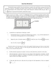
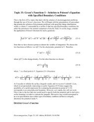
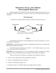
Franck and Hertz devised an arrangement which very neatly measures the firstexcitation potential of mercury by amplifying the effects of collisional excitation by electronswith various energies. To see how this is done, consider the 3-element tube in Figure 2. Youwill heat the cathode by applying a voltage to it, and cause electrons to accelerate by applyinga potential difference V between the cathode and the perforated anode. The tube is filled withmercury vapor so that collisions between electrons and mercury atoms can take place. Most ofthe electrons, whether they make a collision or not, will be drawn to the perforated anode andreturn to the power supply. Some will continue to the collector electrode which is held at asmall retarding potential ∆V (one or two volts negative compared with the anode). Thisretarding potential limits the number of electrons reaching the collector (how?). Theseelectrons then travel from the electrode to a current amplifier or electrometer.to electrometer–∆V0–VCollectorElectrodePerforatedAnodeCathodeHeatingElementFigure 2. Franck-Hertz tubeNow consider the collisions. If the potential difference between cathode and perforatedanode gives the electrons less than the energy needed to collisionally excite a mercury atom,only elastic collisions will occur. However, suppose you increase the potential so that it giveseach electron just enough kinetic energy to excite a mercury atom to the first excited state.Some of the electrons will actually collide with an atom. If the remaining kinetic energy of acolliding electron is insufficient to overcome the retarding potential, such an electron will notreach the collecting electrode. Let's quantify this a little. The required excitation energy can bewritten in terms of the electric potential through which the electron accelerates: E ex = eV exwhere $e$ is the electron charge. If the accelerating potential V has a value between V ex andV ex +∆V , electrons which cause an excitation will not reach the collector unless they gain

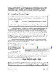
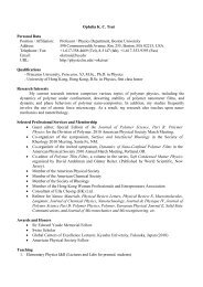
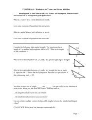
energy from a subsequent collision. As V. is increased above V ex +∆V , electrons will againreach the collector electrode in greater numbers.If one were to measure the current from the electrode as a function of acceleratingpotential, therefore, one would expect to obtain something like Figure 3. The separation ofminima should be equal to the excitation potential (why?).Note that if V. increases above the ionization potential V ion , as it will in yourexperiment, ionization will occur, drawing a huge number of electrons to the anode andcausing a large current to flow toward the power supply. You will prevent this from damagingthe apparatus by connecting a relatively large resistor between anode and power supply. Thiscurrent surge due to ionization will increase the potential across the resistor (consider Ohm'slaw) thus reducing the anode potential to a point which stops the ionization. In practice, theionization only barely gets started.IV exV exV exFigure 3. Current as a function of accelerating potentialPRELAB1. Roughly sketch equipotential lines for the portion of the tube between cathode and anode.Choose a potential V. which is 3.5 times the first excitation potential of mercury. Indicateon the sketch the locations at which you expect the most excitations to occur (note that, andexplain why, each electron can cause up to 3 excitations). You will try to observe this(qualitatively) in the lab.

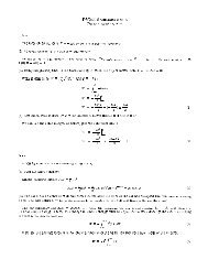
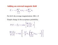
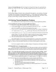
2. At a temperature of 180° C. (the temperature you will use), calculate the mean kinetic energyof a mercury atom in electron volts and discuss whether excitations can occur even if theelectron has considerably less electrostatic energy than V ex . How observable should thistemperature effect be? Note that there is little net kinetic energy transfer from electrons toatoms through elastic collisions; assume that the mean K.E. of mercury atoms (theirtemperature) does not vary with V.3. Why must the gas tube be heated (In what form is mercury at room temperature andpressure)?4. Mercury has a number of excitation potentials, which we did not include in drawing Figure3. What would Figure 3 look like if you included a few of the possible transitions betweenenergy levels shown in Figure 1? Assume all transitions have roughly the same probabilityof occurring. You needn't accurately show the exact energies, but rather just show thegeneral appearance of the plot. (hint: Consider that each transition should cause a `dip' inFigure 3, as should any combination of two or more transitions in one or more atoms,generated by one electron with sufficient energy).collectorelectrodeshielded BNC cableelectrometeror picoAmmeteranodecathodeHg–+A+V–1.5 - 3 V+0-30 VDCPowerSupply–6.3 VACHK6.3 VACTransformer120 VACFigure 4. Schematic diagram

THE APPARATUSA schematic of the circuit which you will use is shown in Figure 4. The power supplyapplies a negative potential to the cathode to accelerate electrons toward the anode. The 10kilohm resistor prevents ionization as discussed above. The electrometer is a current meterwith an amplifier which allows measurement of currents as small as a few picoamperes (1picoampere = 10 -12 amperes). The dotted lines running to the Electrometer represent the outercylindrical conductor of the coaxial cable, just under the plastic insulation, and is connected toground. The perforated anode is held at some small retarding voltage ∆V above ground by twodry cell batteries. The 5 kilohm potentiometer allows you to choose ∆V between 0 and 3 volts.The tube itself is mounted inside a thermostat-regulated oven to maintain the mercury gas inoptimum condition for your measurements.PROCEDURE: PRELIMINARY ADJUSTMENTS1. Plug in the power cord for the oven heater, and insert the thermometer so that the bulb is atthe same height as the center of the tube. A few turns of masking tape around thethermometer will prevent it from falling into the oven. The best oven temperature for thisexperiment is about 180° C., and the oven can be maintained near this temperature by thethermostatic control on the side of it. The thermostat knob is turned {clockwise} toincrease the temperature setting; if turned too far, it will click to indicate that thethermostat is back at its lowest setting. Never turn the knob back (counterclockwise)through this click position. It is all right to make small counterclockwise adjustments aslong as you do not turn through the click position.2. The rest of the apparatus can be connected while the oven heats. The oven front panelcontains a circuit schematic to assist you. Place the oven so that you can see through thewindow in the back {and} make connections to the front panel. Assemble the equipmentas shown in Figure 4. Before plugging in the power cables, turn the power supply controlto its lowest setting.3. Connect a coaxial cable to the Input terminal (the other end should be connected to thecollector electrode, with the black lead grounded). The Output terminal is used foroperating a chart recorder, and will not be used in this experiment.EXPERIMENTS1. Increase the accelerating potential slowly, while watching the value of the collector currentindicated by the electrometer. It will be necessary to use a different range on theelectrometer for the smaller accelerating potentials, but be sure not to `pin' the electrometerneedle to its maximum deflection. Notice the behavior of the electrometer needle as youincrease V. from 0 to about 30 volts. It should show dips in current at several values of V..Ifthe dips in the current are not deep, you may be able to improve matters by making smalladjustments in the oven temperature.

Disconnect the electrometer input and check that the electrometer is zeroed and calibrated.Now, starting again at 0 volts, take data so you will be able to plot collector current as afunction of accelerating potential.To estimate measurement errors, allow the accelerating voltage to remain constant whilethe oven goes through a few cycles (watch the thermometer). Record the fluctuations ofcurrent and temperature (voltage should not change).2. Measure I and V. (just their several minima and maxima) for an additional two or moretemperatures, say 150°, 160°, 170°, 190° C to see if your results are temperature dependent.ANALYSIS & QUESTIONS1. Make a plot of Electrometer current I vs power supply voltage (accelerating potential) V. Dothe maxima and minima all have the same spacing? What is the first excitation potentialV ex of mercury in electron volts? in Joules? Why is the first minimum of I at a voltage thatdiffers from your value of V ex ?2. How would your I vs V. plot appear if the atom energies were {not} quantized?3. Assuming everything else were unchanged, what would be the effect on the I vs V. graph ofthe following: {a.} increasing the retarding potential ∆V. {b.} decreasing the retardingpotential ∆V. {c.} reducing the voltage applied to the cathode. {d.} increasing the density ofmercury in the tube (careful!). Give a brief physical explanation for each effect.4. Do higher excitations (second, third, etc. excited states) appear in your I vs V. plot?Comment briefly in light of your answer to prelab question 4.5. Do the acceleration voltages for minimum current depend on temperature? How about theirspacing, V ex ? Do the values of maximum and minimum current themselves depend ontemperature? What physical reasons can you give for the temperature dependences youobserve?6. Explain what occurs in the tube at potentials corresponding to the second dip in current inyour plot.7. (optional) Explain the bright bluish spot. What is occurring to produce all those emissionlines? (Hint: Consider ionization. Why doesn't the 10 kΩ resistor stop it completely? Hint 2:The rating of 6.3V on the transformer is a root mean squared value, and in addition may beexceeded slightly.)