Statistical physics

1Statistical Thermodynamics - Fall 2009Professor Dmitry GaraninStatistical physicsOctober 24, 2012I. PREFACEStatistical physics considers systems of a large number of entities (particles) such as atoms, molecules, spins, etc. Forthese system it is impossible and even does not make sense to study the full microscopic dynamics. The only relevantinformation is, say, how many atoms have a particular energy, then one can calculate the observable thermodynamicvalues. That is, one has to know the distribution function of the particles over energies that defines the macroscopicproperties. This gives the name statistical physics and defines the scope of this subject.The approach outlined above can be used both at and off equilibrium. The branch of physics studying nonequilibriumsituations is called kinetics. The equilibrium situations are within the scope of statistical physics in thenarrow sense that belongs to this course. It turns out that at equilibrium the energy distribution function has anexplicit general form and the only problem is to calculate the observables.The formalism of statistical physics can be developed for both classical and quantum systems. The resulting energydistribution and calculating observables is simpler in the classical case. However, the very formulation of the method ismore transparent within the quantum mechanical formalism. In addition, the absolute value of the entropy, includingits correct value at T → 0, can only be obtained in the quantum case. To avoid double work, we will consideronly quantum statistical physics in this course, limiting ourselves to systems without interaction. The more generalquantum results will recover their classical forms in the classical limit.II.BASIC DEFINITIONS AND ASSUMPTIONS OF QUANTUM STATISTICAL PHYSICSFrom quantum mechanics follows that the states of the system do not change continuously (like in classical physics)but are quantized. There is a huge number of discrete quantum states with corresponding energy values being the mainparameter characterizing these states. It is the easiest to formulate quantum statistics for systems of noninteractingparticles, then the results can be generalized. In the absence of interaction, each particle has its own set of quantumstates in which it can be at the moment, and for identical particles these sets of states are identical. The particlescan be distributed over their own quantum states in a great number of different ways, the so-called realizations. Eachrealization of this distribution is called microstate of the system. As said above, the information contained in themicrostates is excessive, and the only meaningful information is how many particles N i are in a particular quantumstate i. These numbers N i specify what in statistical physics is called macrostate. If these numbers are known, theenergy and other quantities of the system can be found. It should be noted that the statistical macrostate containsmore information than the macroscopic physical quantities that follow from it.For a large number of particles, each macrostate k can be realized by a very large number w k of microstates, theso-called thermodynamic probability. The main assumption of statistical physics is that all microstates occur withthe same probability. Then the probability of the macrostate k is simply proportional to w k . One can introduce thetrue probability of the macrostate k asp k = w kΩ ,Ω ≡ ∑ kw k . (1)The true probability is normalized by 1:1 = ∑ kp k . (2)Both w k and p k depend on the whole set of N i such asp k = p k (N 1 , N 2 , . . .) . (3)

This dependence will be specified below. For an isolated system the number of particles N and the energy U areconserved, thus the numbers N i satisfy the constraints∑N i = N, (4)i∑N i ε i = U, (5)where ε i is the energy of the particle in the state i. This limits the variety of the macroscopic states k.The number of particles ¯N i averaged over all macrostates k has the formi2¯N i = ∑ kN (k)i p k , (6)where N ik is the number of particles in the microstate i corresponding to the macrostate k. For each macrostate thethermodynamic probabilities differ by a large amount. Then macrostates having small p k practically never occur, andthe state of the system is dominated by macrostates with the largest p k . Consideration of particular models showsthat the maximum of p k is very sharp for large number of particles, whereas N (k)i is a smooth function of k. In thiscase Eq. (6) becomes¯N i∼ = N(k max)i∑kp k = N (kmax)i , (7)where the value k max corresponds to the maximum of p k .In the case of large N, the dominating true probability p k should be found by maximization with respect to all N iobeying the two constraints above.III.TWO-STATE PARTICLES (COIN TOSSING)A tossed coin can land in two positions: Head up or tail up. Considering the coin as a particle, one can say thatthis particle has two “quantum” states, 1 corresponding to the head and 2 corresponding to the tail. If N coins aretossed, this can be considered as a system of N particles with two quantum states each. The microstates of the systemare specified by the states occupied by each coin. As each coin has 2 states, there are totalΩ = 2 N (8)microstates. The macrostates of this system are defined by the numbers of particles in each state, N 1 and N 2 . Thesetwo numbers satisfy the constraint condition (4), i.e., N 1 + N 2 = N. Thus one can take, say, N 1 as the number klabeling macrostates. The number of microstates in one macrostate (that is, the mumber of different microstates thatbelong to the same macrostate) is given by( )N! Nw N1 =N 1 !(N − N 1 )! = . (9)N 1This formula can be derived as follows. We have to pick N 1 particles to be in the state 1, all others will be in the state2. How many ways are there to do this? The first “0” particle can be picked in N ways, the second one can be pickedin N − 1 ways since we can choose of N − 1 particles only. The third “1” particle can be picked in N − 2 differentways etc. Thus one obtains the number of different ways to pick the particles iswhere the factorial is defined byN × (N − 1) × (N − 2) × . . . × (N − N 1 + 1) =N!(N − N 1 )! , (10)N! ≡ N × (N − 1) × . . . × 2 × 1, 0! = 1. (11)The expression in Eq. (10) is not yet the thermodynamical probability w N1 because it contains multiple counting ofthe same microstates. The realizations, in which N 1 “1” particles are picked in different orders, have been counted asdifferent microstates, whereas they are the same microstate. To correct for the multiple counting, one has to divide

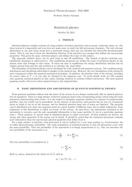
3w( N1) / w(N/ 2)N = 4N = 16N = 1000( N1 − N / 2) /( N / 2)FIG. 1: Binonial distribution for an ensemble of N two-state systems.by the number of permutations N 1 ! of the N 1 particles that yields Eq. (9). One can check that the condition (1) issatisfied,N∑N 1=0w N1 =N∑N 1=0N!N 1 !(N − N 1 )! = 2N . (12)The thermodynamic probability w N1 has a maximum at N 1 = N/2, half of the coins head and half of the coins tail.This macrostate is the most probable state. Indeed, as for an individual coin the probabilities to land head up andtail up are both equal to 0.5, this is what we expect. For large N the maximum of w N1 on N 1 becomes sharp.To prove that N 1 = N/2 is the maximum of w N1 , one can rewrite Eq. (9) in terms of the new variable p = N 1 −N/2asw N1 =N!(N/2 + p)!(N/2 − p)! . (13)One can see that w p is symmetric around N 1 = N/2, i.e., p = 0. Working out the ratioone can see that N 1 = N/2 is indeed the maximum of w N1 .w N/2±1 (N/2)!(N/2)!=w N/2 (N/2 + 1)!(N/2 − 1)! = N/2 < 1, (14)N/2 + 1IV.STIRLING FORMULA AND THERMODYNAMIC PROBABILITY AT LARGE NAnalysis of expressions with large factorials is simplified by the Stirling formulaN! ∼ = √ ( ) N N2πN . (15)e

4In particular, Eq. (13) becomeswherew N1∼ =√2πN (N/e)N√2π (N/2 + p) [(N/2 + p) /e]N/2+p √ 2π (N/2 − p) [(N/2 − p) /e] N/2−p==√2πN√√1 − ( 2pN11 − ( 2pN) 2 (1 +2pN) 2N N(N/2 + p) N/2+p (N/2 − p) N/2−pw N/2) N/2+p (1 −2pN) N/2−p, (16)w N/2∼ =√2πN 2N (17)is the maximal value of the thermodynamic probability. Eq. (16) can be expanded for p ≪ N. Since p enters both thebases and the exponents, one has to be careful and expand the logarithm of w N1 rather than w N1 itself. The squareroot term in Eq. (16) can be discarded as it gives a negligible contribution of order p 2 /N 2 . One obtainsln w N1∼ = ln wN/2 −( N2 + p )ln(1 + 2pN( ) [ N∼= ln w N/2 −2 + p 2pN − 1 2)−( 2pN( N2 − p )ln) 2](1 − 2pN)( ) [ N−2 − p − 2pN − 1 2( ) ] 2 2pNand thus∼= ln w N/2 − p − 2p2N + p2N + p − 2p2N + p2N= ln w N/2 − 2p2Nw N1∼ = wN/2 exp(18)) (− 2p2 . (19)NOne can see that w N1 becomes very small if |p| ≡ |N 1 − N/2| √ N that is much smaller than N for large N. Thatis, w N1 is small in the main part of the interval 0 ≤ N 1 ≤ N and is sharpy peaked near N 1 = N/2.V. MANY-STATE PARTICLESThe results obtained in Sec. III for two-state particles can be generalized for n-state particles. We are looking forthe number of ways to distribute N particles over n boxes so that there are N i particles in ith box. That is, we lookfor the number of microstates in the macrostate described by the numbers N i . The result is given byw =N!N 1 !N 2 ! . . . N n ! = N!∏ ni=1 N i! . (20)This formula can be obtained by using Eq. (9) successively. The number of ways to put N 1 particles in box 1 and theother N − N 1 in other boxes is given by Eq. (9). Then the number of ways to put N 2 particles in box 2 is given bya similar formula with N → N − N 1 (there are only N − N 1 particles after N 1 particles have been put in box 1) andN 1 → N 2 . These numbers of ways should multiply. Then one considers box 3 etc. until the last box n. The resultingnumber of microstates isw =N!N 1 !(N − N 1 )! × (N − N 1 )!N 2 !(N − N 1 − N 2 )! × (N − N 1 − N 2 )!N 3 !(N − N 1 − N 2 − N 3 )! ×. . . × (N n−2 + N n−1 + N n )!N n−2 ! (N n−1 + N n )!× (N n−1 + N n )!N n−1 !N n !× N n!N n !0! . (21)In this formula, all numerators except for the first one and all second terms in the denominators cancel each other, sothat Eq. (20) follows.

The Schrödinger equation can be formulated both for single particles and the systems of particles. In this course wewill restrict ourselves to single particles. In this case the notation ε will be used for single-particle energy levels insteadof E. One can see that Eq. (24) is a second-order linear differential equation. It is an ordinary differential equationin one dimension and partial differential equation in two and more dimensions. If there is a potential energy, this isa linear differential equation with variale coefficients that can be solved analytically only in special cases. In the caseU = 0 this is a linear differential equation with constant coefficients that is easy to solve analytically.An important component of the quantum formalism is boundary conditions for the wave function. In particular, fora particle inside a box with rigid walls the boundary condition is Ψ=0 at the walls, so that Ψ (r) joins smoothly withthe value Ψ (r) = 0 everywhere outside the box. In this case it is also guaranteed that |Ψ (r)| 2 is integrable and Ψ canbe normalized according to Eq. (26). It turns out that the solution of Eq. (24) that satisfies the boundary conditionsexists only for a discrete set of E values that are called eigenvalues. The corresponding Ψ are calles eigenfunctions,and all together is called eigenstates. Eigenvalue problems, both for matrices and differential operators, were known inmathematics before the advent of quantum mechanics. The creators of quantum mechanics, mainly Schrödinger andHeisenberg, realised that this mathematical formalism can accurately describe quantization of energy levels observed inexperiments. Whereas Schrödinger formlated his famous Schrödinger equation, Heisenberg made a major contributioninto description of quantum systems with matrices.6B. Energy levels of a particle in a boxAs an illustration, consider a particle in a one-dimensional rigid box, 0 ≤ x ≤ L. In this case the momentum becomesand Eq. (24) takes the formand can be represented as− 2ˆp = −i ddxd 2(29)Ψ(x) = εΨ(x) (30)2m dx2 d 2dx 2 Ψ(x) + k2 Ψ(x) = 0,k 2 ≡ 2mε 2 . (31)The solution of this equation satisfying the boundary conditions Ψ(0) = Ψ(L) = 0 has the formΨ ν (x) = A sin (k ν x) , k ν = π ν, ν = 1, 2, 3, . . . (32)Lwhere eigenstates are labeled by the index ν. The constant A following from Eq. (26) is A = √ 2/L. The energyeigenvalues are given byε n = 2 k 2 ν2m = π2 2 ν 22mL 2 . (33)One can see the the energy ε is quandratic in the momentum p = k (de Broglie relation), as it should be, butthe energy levels are discrete because of the quantization. For very large boxes, L → ∞, the energy levels becomequasicontinuous. The lowest-energy level with ν = 1 is called the ground state.For a three-dimensional box with sides L x , L y , and L z a similar calculation yields the energy levels parametrizedby the three quantum numbers ν x , ν y , and ν z :()ε νx,ν y,ν z= π2 2 ν 2 x2m L 2 + ν2 yx L 2 + ν2 zy L 2 . (34)zHere the ground state corresponds to ν x = ν y = ν z = 1. One can order the states in increasing ε and number themby the index j, the ground state being j = 1. If L x = L y = L z = L, thenε νx ,ν y ,ν z= π2 2 (ν22mL 2 x + ν 2 y + ν 2 ) π 2 2 ν 2z =2mL 2 (35)and the same value of ε j can be realized for different sets of ν x , ν y , and ν z , for instance, (1,5,12), (5,12,1), etc. Thenumber of different sets of (ν x , ν y , ν z ) having the same ε j is called degeneracy and is denoted as g j . States with ν x =ν y = ν z have g j = 1 and they are called non-degenerate. If only two of the numbers ν x , ν y , and ν z coincide, thedegeneracy is g j = 3. If all numbers are different, g j = 3! = 6. If one sums over the energy levels parametrized by j,one has to multiply the summands by the corresponding degeneracies.

7C. Density of statesFor systems of a large size and thus very finely quantized states, one can define the density of states ρ(ε) as thenumber of energy levels dn ε in the interval dε, that is,dn ε = ρ(ε)dε. (36)It is convenient to start calculation of ρ(ε) by introducing the number of states dn νx ν y ν zdν x dν y dν z , considering ν x , ν y , and ν z as continuous. The result obviously isin the “elementary volume”dn νx ν y ν z= dν x dν y dν z , (37)that is, the corresponding density of states is 1. Now one can rewrite Eq. (34) in the formwhereε = π2 22m(˜ν2x + ˜ν 2 y + ˜ν 2 z)=π 2 2˜ν 22m , (38)˜ν x ≡ ν xL x. (39)The advantage of using this variable is that the vector ˜ν = (˜ν x , ˜ν y , ˜ν z ) is proportional to the momentum p, thusε ∝ ˜ν 2 . Eq. (37) becomesdn˜νx˜ν y ˜ν z= V d˜ν x d˜ν y d˜ν z , V = L x L y L z (40)And after that one can go over to the number of states within the shell d˜ν, as was done for the distribution functionof the molecules over velocities. Taking into account that ˜ν x , ˜ν y , and ˜ν z are all positive, this shell is not a completespherical shell but 1/8 of it. ThusThe last step is to change the variable from ˜ν to ε using Eq. (38). Withdn˜ν = V π 2 ˜ν2 d˜ν. (41)˜ν 2 = 2mπ 2 2 ε,˜ν = √2mπ 2 2 √ ε,d˜νdε = 1 √2m 1 √ε2 π 2 2 (42)one obtainsdn ε = π 4 V ( 2mπ 2 2 ) 3/2√ εdε, (43)that is, in Eq. (36)ρ(ε) =V(2π) 2 ( 2m 2 ) 3/2√ ε. (44)VIII.BOLTZMANN DISTRIBUTION AND CONNECTION WITH THERMODYNAMICSIn this section we obtain the distribution of particles over the n energy levels as the most probable macrostate bymaximizing its thermodynamic probability w. We label quantum states by the index i and use Eq. (20). The taskis to find the maximum of w with respect to all N i that satisfy the constraints (4) and (5). Practically it is moreconvenient to maximize ln w than w itself. Using the method of Lagrange multipliers, one searches for the maximumof the target functionΦ(N 1 , N 2 , · · · , N n ) = ln w + αn∑N i − βi=1n∑ε i N i . (45)i=1

Here α and β are Lagrange multipliers with (arbitrary) signs chosen anticipating the final result.satisfies8The maximum∂Φ∂N i= 0, i = 1, 2, . . . , n. (46)As we are interested in the behavior of macroscopic systems with N i ≫ 1, the factorials can be simplified with thehelp of Eq. (15) that takes the formNeglecting the relatively small last term in this expression, one obtainsΦ ∼ = ln N! −ln N! ∼ = N ln N − N + ln √ 2πN. (47)n∑N j ln N j +j=1n∑n∑N j + α N j − βj=1j=1n∑ε j N j . (48)In the derivatives ∂Φ/∂N i , the only contribution comes from the terms with j = i in the above expression. Oneobtains the equationsthat yieldj=1∂Φ∂N i= − ln N i + α − βε i = 0 (49)N i = e α−βε i, (50)the Boltzmann distribution.The Lagrange multipliers can be found from Eqs. (4) and (5) in terms of N and U. Summing Eq. (50) over i, oneobtainsN = e α Z, α = ln (N/Z) , (51)wheren∑Z = e −βε i(52)i=1is the so-called partition function (German Zustandssumme) that plays a major role in statistical physics.eliminating α from Eq. (50) yieldsThen,N i = N Z e−βε i. (53)After that for the internal energy U one obtainsorU =n∑ε i N i = N Zi=1n∑ε i e −βεi = − N Zi=1∂Z∂β(54)U = −N ∂ ln Z∂β . (55)This formula implicitly defines the Lagrange multiplier β as a function of U.The statistical entropy, Eq. (22), within the Stirling approximation becomes)n∑S = k B ln w = k B(N ln N − N i ln N i . (56)Inserting here Eq. (50) and α from Eq. (51), one obtainsSk B= N ln N −i=1n∑N i (α − βε i ) = N ln N − αN + βU = N ln Z + βU, (57)i=1

Let us show now that β is related to the temperature. To this purpose, we differentiate S with respect to U keepingN = const :1 ∂Sk B ∂U = N ∂ ln Z∂U+ U ∂β∂U + β = N ∂ ln Z ∂β∂β ∂U + U ∂β + β. (58)∂UHere according to Eq. (55) the first and second terms cancel each other leading to∂S∂U = k Bβ. (59)Note that the energies of quantum states ε i depend on the geometry of the system. In particular, for quantum particlesin a box ε i depend on L x , L y , and L z according to Eq. (34). In the differentiation over U above, ε i were kept constant.From the thermodynamical point of view, this amounts to differentiating over U with the constant volume V. Recallingthe thermodynamic formula( ) ∂S= 1 (60)∂UVTand comparing it with Eq. (59), one identifiesβ = 1k B T . (61)Thus Eq. (55) actually defines the internal energy as a function of the temperature. Now from Eq. (57) one obtainsthe statistical formula for the free energyF = U − T S = −Nk B T ln Z. (62)One can see that the partition function Z contains the complete information of the system’s thermodynamics sinceother quantities such as pressure P follow from F.9IX.STATISTICAL THERMODYNAMICS OF THE IDEAL GASIn this section we demonstrate how the results for the ideal gas, previously obtained within the molecular theory,follow from the more general framework of statistical physics in the preceding section. Consider an ideal gas in asufficiently large container. In this case the energy levels of the system, see Eq. (34), are quantized so finely that onecan introduce the density of states ρ (ε) defined by Eq. (36). The number of particles in quantum states within theenergy interval dε is the product of the number of particles in one state N(ε) and the number of states dn ε in thisenergy interval. With N(ε) given by Eq. (53) one obtainsdN ε = N(ε)dn ε = N Z e−βε ρ (ε) dε. (63)For finely quantized levels one can replace summation in Eq. (52) and similar formulas by integration as∑ˆ. . . ⇒ dερ (ε) . . . (64)Thus for the partition function (52) one hasFor quantum particles in a rigid box with the help of Eq. (44) one obtainsZ =V ( ) 3/2 ˆ 2m ∞(2π) 2 20iˆZ = dερ (ε) e −βε . (65)dε √ εe −βε =V ( ) 3/2 √ ( ) 3/2 2m π(2π) 2 2 2β = V mkB T3/2 2π 2 . (66)Using the classical relation ε = mv 2 /2 and thus dε = mvdv, one can obtain the formula for the number of particles inthe speed interval dvdN v = Nf(v)dv, (67)

10where the speed distribution function f(v) is given byf(v) ==1 Z e−βε ρ (ε) mv = 1 V( 2π2mk B T( ) 3/2 m4πv 2 exp(− mv22πk B T2k B T) 3/2V( ) 3/2 √ 2m m(2π) 2 2 v mv e−βε2). (68)This result coincides with the Maxwell distribution function obtained earlier from the molecular theory of gases. ThePlank’s constant that links to quantum mechanics disappeared from the final result.The internal energy of the ideal gas is its kinetic energyU = N¯ε, (69)¯ε = m¯v 2 /2 being the average kinetic energy of an atom. The latter can be calculated with the help of the speeddistribution function above, as was done in the molecular theory of gases. The result has the form¯ε = f 2 k BT, (70)where in our case f = 3 corresponding to three translational degrees of freedom. The same result can be obtainedfrom Eq. (55)U = −N ∂ ln Z∂β= −N ∂ ( ) 3/2 m∂β V ln 2π 2 = 3 β 2 N ∂∂β ln β = 3 2 N 1 β = 3 2 Nk BT. (71)After that the known result for the heat capacity C V = (∂U/∂T ) Vfollows.The pressure P is defined by the thermodynamic formula( ) ∂FP = −∂V. (72)With the help of Eqs. (62) and (66) one obtainsP = Nk B T ∂ ln Z∂VT= Nk B T ∂ ln V∂Vthat amounts to the equation of state of the ideal gas P V = Nk B T.= Nk BTV(73)X. STATISTICAL THERMODYNAMICS OF HARMONIC OSCILLATORSConsider an ensemble of N identical harmonic oscillators, each of them described by the HamiltonianĤ = ˆp22m + kx22 . (74)Here the momentum operator ˆp is given by Eq. (29) and k is the spring constant. This theoretical model can describe,for instance, vibrational degrees of freedom of diatomic molecules. In this case x is the elongation of the chemicalbond between the two atoms, relative to the equilibrium bond length. The stationary Schrödinger equation (24) fora harmonic oscillator becomes(− 2 d 2 )2m dx 2 + kx2 Ψ(x) = εΨ(x). (75)2The boundary conditions for this equation require that Ψ(±∞) = 0 and the integral in Eq. (26) converges. In contrastto Eq. (30), this is a linear differential equation with a variable coefficient. Such differential equations in general donot have solutions in terms of known functions. In some cases the solution can be expressed through special functionssuch as hypergeometrical, Bessel functions, etc. Solution of Eq. (75) can be found but this task belongs to quantummechanics courses. The main result that we need here is that the energy eigenvalues of the harmonic oscillator havethe form(ε ν = ω 0 ν + 1 ), ν = 0, 1, 2, . . . , (76)2

12C /( NkB )k BT/( hω ) 0FIG. 2: Heat capacity of harmonic oscillators.The heat capacity is defined byC = dUdT = N ω (0−21sinh 2 [ω 0 /(2k B T )]) (− ω ) ( ) 20ω0 /(2k B T )2k B T 2 = Nk B . (87)sinh [ω 0 /(2k B T )]This formula has limiting casesC ∼ ={ ( ) 2 ( )ωNk 0 B k BT exp − ω0k BT, k B T ≪ ω 0Nk B , k B T ≫ ω 0 .(88)One can see that at high temperatures the heat capacity can be written asC = f 2 Nk B, (89)where the effective number of degrees of freedom for an oscillator is f = 2. The explanation of the additional factor2 is that the oscillator has not only the kinetic, but also the potential energy, and the average values of these twoenergies are the same. Thus the total amount of energy in a vibrational degree of freedom doubles with respect to thetranslational and rotational degrees of freedom.At low temperatures the vibrational heat capacity above becomes exponentially small. One says that vibrationaldegrees of freedom are getting frozen out at low temperatures.The average quantum number of an oscillator is given byn ≡ ⟨ν⟩ = 1 ZUsing Eq. (76), one can calculate this sum as followsn = 1 Z∞∑ν=0( 12 + ν )e −βεν − 1 Z∞∑ν=0Finally with the help of Eq. (84), one finds1= 1 12 e−βεν ω 0 Z∞∑ν=0∞∑νe −βεν . (90)ν=0ε ν e −βεν − Z 2Z = − 1 1 ∂Zω 0 Z ∂β − 1 2 = U − 1 Nω 0 2 . (91)n =1e βω0 − 1 = 1exp [ω 0 /(k B T )] − 1(92)

13so thatU = Nω 0( 12 + n ). (93)At low temperatures, k B T ≪ ω 0 , the average quantum number n becomes exponentially small. This means that theoscillator is predominantly in its ground state, ν = 0. At high temperatures, k B T ≫ ω 0 , Eq. (92) yieldsn ∼ = k BTω 0(94)that has the same order of magnitude as the top populated quantum level number ν ∗ given by Eq. (86).To conclude this section, let us reproduce the classical high-temperature results by a simpler method. At hightemperatures, many levels are populated and the distribution function e −βε νonly slightly changes from one level tothe other. Indeed its relative change ise −βε ν− e −βε ν+1e −βε ν= 1 − e −β(εν+1−εν) = 1 − e −βω0 ∼ = 1 − 1 + βω 0 = ω 0k B T≪ 1. (95)In this situation one can replace summation in Eq. (77) by integration using the rule in Eq. (64). The density ofstates ρ (ε) for the harmonic oscillator can be easily found. The number of levels dn ν in the interval dν isdn ν = dν (96)(that is, there is only one level in the interval dν = 1). Then, changing the variables with the help of Eq. (76), onefinds the number of levels dn ε in the interval dε asdn ε = dν ( ) −1 dεdε dε = dε = ρ (ε) dε, (97)dνwhereρ (ε) = 1ω 0. (98)One actually can perform a one-line calculation of the partition function Z via integration. Considering ν as continuous,one writesZ =ˆ ∞0dνe −βε =ˆ ∞0dε dνdε e−βε = 1ω 0ˆ ∞0dεe −βε = 1ω 0 β = k BTω 0. (99)One can see that this calculation is in accord with Eq. (98). Now the internal energy U is given bythat coincides with the second line of Eq. (85).U = −N ∂ ln Z∂β = −N ∂ ln 1 β + . . .= N ∂ ln β + . . . = N ∂β∂β β = Nk BT (100)XI.STATISTICAL THERMODYNAMICS OF ROTATORSThe rotational kinetic energy of a rigid body, expressed with respect to the principal axes, readsE rot = 1 2 I 1ω 2 1 + 1 2 I 2ω 2 2 + 1 2 I 3ω 2 3. (101)We will restrict our consideration to the axially symmetric body with I 1 = I 2 = I. In this case E rot can be rewrittenin terms of the angular momentum components L α = I α ω α as followsE rot = L22I + 1 ( 1− 1 )L 22 I 3 I3. (102)In the important case of a diatomic molecule with two identical atoms, then the center of mass is located betweenthe two atoms at the distance d/2 from each, where d is the distance between the atoms. The moment of inertia of

the molecule with respect to the 3 axis going through both atoms is zero, I 3 = 0. The moments of inertia with respectto the 1 and 2 axis are equal to each other:14( ) 2 dI 1 = I 2 = I = 2 × m = 1 2 2 md2 , (103)where m is the mass of an atom. In our case, I 3 = 0, there is no kinetic energy associated with rotation around the 3axis. Then Eq. (102) requires L 3 = 0, that is, the angular momentum of a diatomic molecule is perpendicular to itsaxis.In quantum mechanics L and L 3 become operators. The solution of the stationary Schrödinger equation yieldseigenvalues of L 2 , L 3 , and E rot in terms of three quantum numbers l, m, and n. These eigenvalues are given byˆL 2 = 2 l(l + 1), l = 0, 1, 2, . . . (104)ˆL 3 = n, m, n = −l, −l + 1, . . . , l − 1, l (105)andE rot = 2 l(l + 1)2I+ 22( 1I 3− 1 I)n 2 (106)that follows by substitution of Eqs. (104) and (105) into Eq. (102). One can see that the results do not depend onthe quantum number m and there are 2l + 1 degenerate levels because of this. Indeed, the angular momentum ofthe molecule ˆL can have 2l + 1 different projections on any axis and this is the reason for the degeneracy. Further,the axis of the molecule can have 2l + 1 different projections on ˆL parametrized by the quantum number n. In thegeneral case I 3 ≠ I these states are non-degenerate. However, they become degenerate for the fully symmetric body,I 1 = I 2 = I 3 = I. In this caseE rot = 2 l(l + 1)2I(107)and the degeneracy of the quantum level l is g l = (2l + 1) 2 . For the diatomic molecule I 3 = 0, and the only acceptablevalue of n is n = 0. Thus one obtains Eq. (107) again but with the degeneracy g l = 2l + 1.The rotational partition function both for the symmetric body and for a diatomic molecule is given byZ = ∑ lg l e −βε l, g l = (2l + 1) ξ , ξ ={2, symmetric body1, diatomic molecule,(108)where ε l ≡ E rot . In both cases Z cannot be calculated analytically in general. In the general case I 1 = I 2 ≠ I 3 withI 3 ≠ 0 one has to perform summation over both l and n.In the low-temperature limit, most of rotators are in their ground state l = 0, and very few are in the first excitedstate l = 1. Discarding all other values of l, one obtains)Z ∼ = 1 + 3 ξ exp(− β2(109)Iat low temperatures. The rotational internal energy is given byU = −N ∂ ln Z( ) ( )2= 3ξ∂β I exp − β2 = 3 ξ 2I I exp −2Ik B T(110)and it is exponentially small. The heat capacity isC V =( ) ∂U∂TV( ) = 3 ξ 2 2 )k B exp(− 2Ik B T Ik B Tand it is also exponentially small.In the high-temperature limit, very many energy levels are thermally populated, so that in Eq. (108) one can replacesummation by integration. Withg l∼ = (2l) ξ , ε l ≡ ε ∼ = 2 l 22I , ∂ε∂l = 2 lI , ∂l∂ε = I √ √2 I 2 2Iε = 2 2 (112)ε(111)

15C /( NkB )Fully symmetric bodyDiatomic molecule2IT/ h2FIG. 3: Rotational heat capacity of a fully symmetric body and a diatomic molecule.one hasand furtherZ ∼ =ˆ ∞0dl g l e −βε l ∼ = 2ξˆ ∞0ˆ ∞dl l ξ e −βε l= 2 ξ0dε ∂l∂ε lξ e −βε (113)√ ˆZ ∼ I ∞= 2 ξ 2 2 dε√ 1 ( ) ξ/2 ( ) (ξ+1)/2 ˆ 2IεI ∞ε 2 e −βε = 2 (3ξ−1)/2 2 dε ε (ξ−1)/2 e −βεNow the internal energy is given bywhereas the heat capacity is0( ) (ξ+1)/2 ˆ I∞= 2 (3ξ−1)/2 β 2 dx x (ξ−1)/2 e −x ∝ β −(ξ+1)/2 . (114)0U = −N ∂ ln Z∂β = ξ + 12 N ∂ ln β∂β = ξ + 12 N 1 β = ξ + 12 Nk BT, (115)C V =( ) ∂U∂TV0= ξ + 12 Nk B. (116)In these two formulas, f = ξ + 1 is the number of degrees of freedom, f = 2 for a diatomic molecule and f = 3 for afully symmetric rotator. This result confirms the principle of equidistribution of energy over the degrees of freedomin the classical limit that requires temperatures high enough.To conclude this section, let us calculate the partition function classically at high temperatures. The calculationcan be performed in the general case of all moments of inertia different. The rotational energy, Eq. (101), can bewritten asE rot = L2 12I 1+ L2 22I 2+ L2 32I 3. (117)The dynamical variables here are the angular momentum components L 1 , L 2 , and L 3 , so that the partition function

16can be obtained by integration with respect to themZ class ===ˆ ∞−∞ˆ ∞−∞dL 1 dL 2 dL 3 exp (−βE rot )( ) ˆ ∞(dL 1 exp − βL2 1× dL 2 exp − βL2 22I 1 −∞(ˆ ∞√2I 1β × 2I 2β × 2I 3β2I 2)ˆ ∞( )× dL 3 exp − βL2 3−∞2I 3) 3dx e −x2 ∝ β −3/2 . (118)−∞In fact, Z class contains some additional coefficients, for instance, from the integration over the orientations of themolecule. However, these coefficients are irrelevant in the calculation of the the internal energy and heat capacity. Forthe internal energy one obtainsU = −N ∂ ln Z∂β= 3 2 N ∂ ln β∂β = 3 2 Nk BT (119)that coincides with Eq. (115) with ξ = 2. In the case of the diatomic molecule the energy has the formThen the partition function becomesE rot = L2 12I 1+ L2 22I 2. (120)Z class ===ˆ ∞−∞ˆ ∞−∞dL 1 dL 2 exp (−βE rot )( ) ˆ ∞(dL 1 exp − βL2 1× dL 2 exp − βL2 22I 1 −∞(ˆ ∞√2I 1β × 2I 2β2I 2)) 2dx e −x2 ∝ β −1 . (121)−∞This leads toU = Nk B T, (122)in accordance with Eq. (115) with ξ = 1.XII.STATISTICAL PHYSICS OF VIBRATIONS IN SOLIDSAbove in Sec. X we have studied statistical mechannics of harmonic oscillators. For instance, a diatomic moleculebehaves as an oscillator, the chemical bond between the atoms periodically changing its length with time in theclassical description. For molecules consisting of N ≥ 2 atoms, vibrations become more complicated and, as a rule,involve all N atoms. Still, within the harmonic approximation (the potential energy expanded up to the second-orderterms in deviations from the equilibrium positions) the classical equations of motion are linear and can be dealt withmatrix algebra. Diagonalizing the dynamical matrix of the system, one can find 3N − 6 linear combinations of atomiccoordinates that dynamically behave as independent harmonic oscillators. Such collective vibrational modes of thesystem are called normal modes. For instance, a hypothetic triatomic molecule with atoms that are allowed to movealong a straight line has 2 normal modes. If the masses of the first and third atoms are the same, one of the normalmodes corresponds to antiphase oscillations of the first and third atoms with the second (central) atom being at rest.Another normal mode corresponds to the in-phase oscillations of the first and third atoms with the central atomoscillating in the anti-phase to them. For more complicated molecules normal modes can be found numerically.Normal modes can be considered quantum mechanically as independent quantum oscillators as in Sec. X. Then thevibrational partition function of the molecule is a product of partition functions of individual normal modes and theinternal energy is a sum of internal energies of these modes. The latter is the consequence of the independence of thenormal modes.The solid having a well-defined crystal structure is translationally invariant that simplifies finding normal modes,in spite of a large number of atoms N. In the simplest case of one atom in the unit cell normal modes can be foundimmediately by making Fourier transformation of atomic deviations. The resulting normal modes are sound waves

with different wave vectors k and polarizations (in the simplest case one longitudinal and two equivalent transversemodes). In the sequel, to illustrate basic principles, we will consider only one type of sound waves (say, the longitudinalwave) but we will count it three times. The results can be then generalized for different kinds of waves. For wavevectors small enough, there is the linear relation between the wave vector and the frequency of the oscillationsω k = vk (123)In this formula, ω k depends only on the magnitude k = 2π/λ and not on the direction of k and v is the speed of sound.The acceptable values of k should satisfy the boundary conditions at the boundaries of the solid body. Similarly to thequantum problem of a particle in a potential box with dimentions L x , L y , and L z , one obtains the quantized valuesof the wave vector components k α with α = x, y, zso thatk =k α = π ν αL α, ν = 1, 2, 3, . . . , (124)√√kx 2 + ky 2 + kxz 2 = π ˜ν 2 x + ˜ν 2 y + ˜ν 2 z = π˜ν,17˜ν α ≡ ν αL α. (125)Similarly to the problem of the particle in a box, one can introduce the frequency density of states ρ (ω) via thenumber of normal modes in the frequency interval dωdn ω = ρ (ω) dω. (126)Starting with Eq. (37), one arrives at Eq. (41). Then with the help of ω = vπ˜ν following from Eqs. (123)–(125) oneobtainsthat yields for the frequency density of statesThe total number of normal modes should be 3N:dn ω = 3 × V π d˜ν ˜ν22 dω = 3 × V π 2ρ (ω) =3N = 3 ∑ k1(vπ) 3 ω2 dω (127)3V2π 2 v 3 ω2 . (128)1 = 3 ∑k x ,k y ,k x1. (129)For a body of a box shape N = N x N y N z , so that the above equation splits into the three separate equationsfor α = x, y, z. This results inN α =k α,max∑k α =1∼= ν α,max (130)k α,max = π N αL α= πa, (131)where a is the lattice spacing, that is, the distance between the atoms.As the solid body is macroscopic and there are very many values of the allowed wave vectors, it is convenient toreplace summation my integration and use the density of states:∑. . . ⇒kˆ ωmax0dωρ (ω) . . . (132)At large k and thus ω, the linear dependence of Eq. (123) is no longer valid, so that Eq. (128) becomes invalid aswell. Still, one can make a crude approximation assuming that Eqs. (123) and (128) are valid until some maximalfrequency of the sound waves in the body. The model based on this assumption is called Debye model. The maximalfrequency (or the Debye frequency ω D ) is defined by Eq. (129) that takes the form3N =ˆ ωD0dωρ (ω) . (133)

18With the use of Eq. (128) one obtainswherefrom3N =ˆ ωD0dω3V2π 2 v 3 ω2 = V ω3 D2π 2 v 3 , (134)ω D = ( 6π 2) 1/3 va , (135)where we used (V/N) 1/3 = v 1/30 = a, and v 0 is the unit-cell volume. It is convenient to rewrite Eq. (128) in terms ofω D asρ (ω) = 9N ω2ω 3 . (136)DThe quantum energy levels of a harmonic oscillator are given by Eq. (76). In our case for a k-oscillator it becomes(ε k,νk = ω k ν k + 1 ), ν = 0, 1, 2, . . . (137)2All the k-oscillators contribute additively into the internal energy,U = 3 ∑ ⟨ε k,νk ⟩ = 3 ∑ (ω k ⟨ν k ⟩ + 1 )= 3 ∑ 2kkk(ω k n k + 1 ), (138)2where, similarly to Eq. (92),n k =1exp (βω k ) − 1 . (139)Replacing summation by integration and rearranging Eq. (138), within the Debye model one obtainsU = U 0 +ˆ ωD0dωρ (ω)ωexp (βω) − 1 , (140)where U 0 is the zero-temperature value of U due to the zero-point motion. The integral term in Eq. (140) can becalculated analytically at low and high temperatures.For k B T ≪ ω D , the integral converges at ω ≪ ω D , so that one can extend the upper limit of integration to ∞.One obtainsU = U 0 +ˆ ∞0dωρ (ω)ˆ9N ∞= U 0 +(ω D ) 3 β 4 dxThis result can be written in the formwhereωexp (βω) − 1 = U 0 + 9Nω 3 D0x3e x − 1 = U 0 +is the Debye temperature. The heat capacity is given byC V =ˆ ∞0dω ω 2 ωexp (βω) − 19N π 4(ω D ) 3 β 4 15 = U 0 + 3π45 Nk BT(kB Tω D) 3. (141)( ) 3U = U 0 + 3π4 T5 Nk BT , (142)θ D( ) ∂U∂TVθ D = ω D /k B (143)( ) 3= 12π4 T5 Nk B , T ≪ θ D . (144)θ DAlthough the Debye temperature enters Eqs. (142) and (144), these results are accurate and insensitive to the Debyeapproximation.

19C /( NkB )T 3T / θ DFIG. 4: Temperature dependence of the phonon heat capacity. The low-temperature result C ∝ T 3 (dashed line) holds only fortemperatures much smaller than the Debye temperature θ D.For k B T ≫ ω D , the exponential in Eq. (140) can be expanded for βω ≪ 1. It is, however, convenient to stepback and to do the same in Eq. (138). WIth the help of Eq. (129) one obtainsU = U 0 + 3 ∑ kFor the heat capacity one then obtainsω kβω k= U 0 + 3k B T ∑ k1 = U 0 + 3Nk B T. (145)C V = 3Nk B , (146)k B per each of approximately 3N vibrational modes. One can see that Eqs. (145) and (146) are accurate becausethey do not use the Debye model. The assumption of the Debye model is really essential at intermediate temperatures,where Eq. (140) is approximate.The temperature dependence of the photon heat capacity, following from Eq. (140), is shown in Fig. 4 togetherwith its low-temperature asymptote, Eq. (144), and the high-temperature asymptote, Eq. (146). Because of the largenumerical coefficient in Eq. (144), the law C V ∝ T 3 in fact holds only for the temperatures much smaller than theDebye temperature.XIII.SPINS IN MAGNETIC FIELDMagnetism of solids is in most cases due to the intrinsic angular momentum of the electron that is called spin. Inquantum mechanics, spin is an operator represented by a matrix. The value of the electronic angular momentum iss = 1/2, so that the quantum-mechanical eigenvalue of the square of the electron’s angular momentum (in the unitsof ) isŝ 2 = s (s + 1) = 3/4 (147)c.f. Eq. (104). Eigenvalues of ŝ z , projection of a free spin on any direction z, are given byŝ z = m, m = ±1/2 (148)c.f. Eq. (105). Spin of the electron can be interpreted as circular motion of the charge inside this elementary particle.This results in the magnetis moment of the electronˆµ = gµ B ŝ, (149)

where g = 2 is the so-called g-factor and µ B is Bohr’s magneton, µ B = e/ (2m e ) = 0.927 × 10 −23 J/T. Note thatthe model of circularly moving charges inside the electron leads to the same result with g = 1; The true value g = 2follows from the relativistic quantum theory.The energy (the Hamiltonian) of an electron spin in a magnetic field B has the formĤ = −gµ B ŝ · B, (150)the so-called Zeeman Hamiltonian. One can see that the minimum of the energy corresponds to the spin pointing inthe direction of B. Choosing the z axis in the direction of B, one obtainsĤ = −gµ B ŝ z B. (151)Thus the energy eigenvalues of the electronic spin in a magnetic field with the help of Eq. (148) becomeε m = −gµ B mB, (152)where, for the electron, m = ±1/2.In an atom, spins of all electrons usually combine in a collective spin S that can be greater than 1/2. Thus insteadof Eq. (150) one hasEigenvalues of the projections of Ŝ on the direction of B areĤ = −gµ B Ŝ · B. (153)m = −S, −S + 1, . . . , S − 1, S, (154)all together 2S + 1 different values, c.f. Eq. (104). The 2S + 1 different energy levels of the spin are given by Eq.(152).Physical quantities of the spin are determined by the partition functionwhere ε m is given by Eq. (152) andZ S =S∑m=−Se −βε m=Eq. (155) can be reduced to a finite geometrical progressionS∑m=−S20e my , (155)y ≡ βgµ B B = gµ BBk B T . (156)Z S = e −Sy 2S∑k=0(e y ) k = e −yS e(2S+1)y − 1e y − 1= e(S+1/2)y − e −(S+1/2)ye y/2 − e −y/2=sinh [(S + 1/2)y]. (157)sinh (y/2)For S = 1/2 with the help of sinh(2x) = 2 sinh(x) cosh(x) one can transform Eq. (157) toZ 1/2 = 2 cosh (y/2) . (158)The partition function beng found, one can easily obtain thermodynamic quantities.. For instance, the free energyF is given by Eq. (62),The average spin polarization is defined byWith the help of Eq. (155) one obtainsF = −Nk B T ln Z S = −Nk B T ln⟨S z ⟩ = ⟨m⟩ = 1 Z⟨S z ⟩ = 1 ZS∑m=−Ssinh [(S + 1/2)y]. (159)sinh (y/2)me −βε m. (160)∂Z∂y = ∂ ln Z∂y . (161)

21B S (x)S = 1/215/2S = ∞xFIG. 5: Brillouin function B S(x) for different S.With the use of Eq. (157) and the derivativessinh(x) ′ = cosh(x), cosh(x) ′ = sinh(x) (162)one obtains⟨S z ⟩ = b S (y), (163)whereb S (y) =(S + 1 ) [(coth S + 1 ) ]y − 1 [ ] 122 2 coth 2 y . (164)Usually the function b S (y) is represented in the form b S (y) = SB S (Sy), where B S (x) is the Brillouin function(B S (x) = 1 + 1 ) [(coth 1 + 1 ) ]x − 1 [ ] 12S2S 2S coth 2S x . (165)For S = 1/2 from Eq. (158) one obtains⟨S z ⟩ = b 1/2 (y) = 1 2 tanh y 2(166)and B 1/2 (x) = tanh x. One can see that b S (±∞) = ±S and B S (±∞) = ±1. At zero magnetic field, y = 0, the spinpolarization should vanish. It is immediately seen in Eq. (166) but not in Eq. (163). To clarify the behavior of b S (y)at small y, one can use coth x ∼ = 1/x + x/3 that yieldsIn physical units, this means(b S (y) ∼ = S + 1 ) [ (1( )2 S +1+ S + 1 ) ]y− 1 [ 12 y 2 3 212 y + 1 2[ (= y S + 1 ) 2 ( ] 2 1− =3 2 2)⟨S z ⟩ ∼ =]y3S(S + 1)y. (167)3S(S + 1) gµ B B3 k B T , gµ BB ≪ k B T. (168)

22The average magnetic moment of the spin can be obtained from Eq. (149)⟨µ z ⟩ = gµ B ⟨S z ⟩ . (169)The magnetization of the sample M is defined as the magnetic moment per unit volume. If there is one magneticatom per unit cell and all of them are uniformly magnetized, the magnetization readsM = ⟨µ z⟩v 0= gµ Bv 0⟨S z ⟩ , (170)where v 0 is the unit-cell volume.The internal energy U of a system of N spins can be obtained from the general formula, Eq. (55). The calculationcan be, however, avoided since from Eq. (152) simply followsU = N ⟨ε m ⟩ = −Ngµ B B ⟨m⟩ = −Ngµ B B ⟨S z ⟩ = −Ngµ B Bb S (y) = −Nk B T yb S (y) . (171)In particular, at low magnetic fields (or high temperatures) one hasU ∼ = −NThe magnetic susceptibility per spin is defined byFrom Eqs. (169) and (163) one obtainswhereb ′ S(y) ≡ db S(y)dyFor S = 1/2 from Eq. (166) one obtains(= −S(S + 1)3(gµ B B) 2. (172)k B Tχ = ∂ ⟨µ z⟩∂B . (173)χ = (gµ B) 2k B T b′ S(y), (174)S + 1/2sinh [(S + 1/2) y]) 2 ( ) 2 1/2+. (175)sinh [y/2]b ′ 1/2 (y) = 14 cosh 2 (y/2) . (176)From Eq. (167) follows b ′ S (0) = S(S + 1)/3, thus one obtains the high-temperature limitχ =S(S + 1) (gµ B ) 23 k B T , k BT ≫ gµ B B. (177)In the opposite limit y ≫ 1 the function b ′ S (y) and thus the susceptibility becomes small. The physical reason for thisis that at low temperatures, k B T ≪ gµ B B, the spins are already strongly aligned by the magnetic field, ⟨S z ⟩ ∼ = S,so that ⟨S z ⟩ becomes hardly sensitive to small changes of B. As a function of temperature, χ has a maximum atintermediate temperatures.The heat capacity C can be obtained from Eq. (171) asC = ∂U∂T = −Ngµ BBb ′ S(y) ∂y∂T = Nk Bb ′ S(y)y 2 . (178)One can see that C has a maximum at intermediate temperatures, y ∼ 1. At high temperatures C decreases as 1/T 2 :( ) 2C ∼ S(S + 1) gµB B= Nk B , (179)3 k B Tand at low temperatures C becomes exponentially small, except for the case S = ∞ (see Fig. 6). Finally, Eqs. (174)and (178) imply a simple relation between χ and Cthat does not depend on the spin value S.NχC = T B 2 (180)

23C /( NkB )S = ∞5/21S = 1/2k T /( Sg B)BµBFIG. 6: Temperature dependence of the heat capacity of spins in a magnetic fields with different values of S.XIV.PHASE TRANSITIONS AND THE MEAN-FIELD APPROXIMATIONAs explained in thermodynamics, with changing thermodynamic parameters such as temperature, pressure, etc.,the system can undergo phase transitions. In the first-order phase transitions, the chemical potentials µ of the twocompeting phases become equal at the phase transition line, while on each side of this line they are unequal and onlyone of the phases is thermodynamically stable. The first-order trqansitions are thus abrupt. To the contrast, secondordertransitions are gradual: The so-called order parameter continuously grows from zero as the phase-transition lineis crossed. Thermodynamic quantities are singular at second-order transitions.Phase transitions are complicated phenomena that arise due to interaction between particles in many-particlesystems in the thermodynamic limit N → ∞. It can be shown that thermodynamic quantities of finite systems arenon-singular and, in particular, there are no second-order phase transitions. Up to now in this course we studiedsystems without interaction. Including the latter requires an extension of the formalism of statistical mechanics thatis done in Sec. XV. In such an extended formalism, one has to calculate partition functions over the energy levels ofthe whole system that, in general, depend on the interaction. In some cases these energy levels are known exactly butthey are parametrized by many quantum numbers over which summation has to be carried out. In most of the cases,however, the energy levels are not known analytically and their calculation is a huge quantum-mechanical problem. Inboth cases calculation of the partition function is a very serious task. There are some models for which thermodynamicquantities had been calculated exactly, including models that possess second-order phase transitions. For other models,approximate numerical methods had been developed that allow calculating phase transition temperatures and criticalindices. It was shown that there are no phase transitions in one-dimensional systems with short-range interactions.It is most convenient to illustrate the physics of phase transitions considering magnetic systems, or the systems ofspins introduced in Sec. XIII. The simplest forms of interaction between different spins are Ising interaction −J ij Ŝ iz Ŝ jzincluding only z components of the spins and Heisenberg interaction −J ij Ŝ i · Ŝ j . The exchange interaction J ij followsfrom quantum mechanics of atoms and is of electrostatic origin. In most cases practically there is only interaction Jbetween spins of the neighboring atoms in a crystal lattice, because J ij decreases exponentially with distance. Forthe Ising model, all energy levels of the whole system are known exactly while for the Heisenberg model they are not.In the case J > 0 neighboring spins have the lowest interaction energy when they are collinear, and the state withall spins pointing in the same direction is the exact ground state of the system. For the Ising model, all spins in theground state are parallel or antiparallel with the z axis, that is, it is double-degenerate. For the Heisenberg model thespins can point in any direction in the ground state, so that the ground state has a continuous degeneracy. In bothcases, Ising and Heisenberg, the ground state for J > 0 is ferromagnetic.The nature of the interaction between spins considered above suggests that at T → 0 the system ⟩∣ should fall into its∣ ∣∣ground state, so that thermodynamic averages of all spins approach their maximal values, ∣⟨Ŝi → S. With increasing

⟩∣∣ ∣∣temperature, excited levels of the system become populated and the average spin value decreases, ∣⟨Ŝi < S. At hightemperatures all energy levels become populated, so that neighboring spins can have all possible orientations withrespect to each other. In this case, if there is no external magnetic field acting on the spins (see Sec. XIII), the averagespin value should be exactly zero, because there as many spins pointing in one direction as there are the spins pointingin the other direction. This is why the high-temperature state is called symmetric state. If now the temperature islowered, there should be a phase transition temperature T C (the Curie temperature for ferromagnets) below whichthe order parameter (average spin value) becomes nonzero. Below T C the symmetry of the state is spontaneouslybroken. This state is called ordered state. Note that if there is an applied magnetic field, it will break the symmetry bycreating ⟩∣a nonzero spin average at all temperatures, so that there is no sharp phase transition, only a gradual increase∣ ∣∣of ∣⟨Ŝi as the temperature is lowered.Although ⟩∣ the scenario outlined above looks persuasive, there are subtle effects that may preclude ordering and∣ ∣∣ensure ∣⟨Ŝi = 0 at all nonzero temperatures. As said above, ordering does not occur in one dimension (spin chains)for both Ising and Heisenberg models. In two dimensions, Ising model shows a phase transition, and the analyticalsolution of the problem exists and was found by Lars Osager. However, two-dimensional Heisenberg model does notorder. In three dimensions, both Ising and Heisenberg models show a phase transition and no analytical solution isavailable.24A. The mean-field approximation for ferromagnetsWhile a rigorous solution of the problem of phase transition is very difficult, there is a simple approximate solutionthat captures the physics of phase transitions as described above and provides qualitatively correct results in mostcases, including three-dimensional systems. The idea of this approximate solution is to reduce the original many-spinproblem to an effective self-consistent one-spin problem by considering one spin ⟩(say i) and replacing other spins in theinteraction by their average thermodynamic values, −J ij Ŝ i · Ŝ j ⇒ −J ij Ŝ i ·⟨Ŝj . One can see that now the interactionterm has mathematically the same form as the term describing interaction of a spin with the applied magnetic field,Eq. (153). Thus one can use the formalism of Sec. (XIII) to solve the problem analytically. This aproach is calledmean field approximation (MFA) or molecular field approximation and it was first suggested by Weiss for ferromagnets.The effective one-spin Hamiltonian within the MFA is similar to Eq: (153) and has the form(⟩)Ĥ = −Ŝ· gµ B B + Jz⟨Ŝ + 1 ⟨Ŝ⟩ 22 Jz , (181)where z is the number of nearest neigbors for a spin in the lattice (z = 6 for the simple cubic lattice). Here the last⟩⟩⟨Ŝ⟩ 2term ensures that the replacement Ŝ ⇒⟨Ŝ in⟨ŜĤ yields Ĥ = − ·gµ B B − (1/2)Jz that becomes the correct∣ ∣∣ground-state energy at T = 0 where ∣⟨Ŝ⟩∣= S. For the Heisenberg model, in the presence of a whatever weak appliedfield B the ordering will occur in the direction of B. Choosing the z axis in this direction, one can simplify Eq. (181)to(⟩)Ĥ = − gµ B B + Jz⟨Ŝz Ŝz + 1 ⟩ 2 ⟨Ŝz2 Jz . (182)The same mean-field Hamilotonian is valid for the Ising model as well, if the magnetic field is applied along the zaxis. Thus, within the MFA (but not in general!) Ising and Heisenberg models are equivalent. The energy levelscorresponding to Eq. (182) are(⟩)ε m = − gµ B B + Jz⟨Ŝz m + 1 ⟩ 2 ⟨Ŝz2 Jz , m = −S, −S + 1, . . . , S − 1, S. (183)Now, after calculation of the partition function Z, Eq. (155), one arrives at the free energy per spinF = −k B T ln Z = 1 2 Jz ⟨Ŝz⟩ 2− kB T lnsinh [(S + 1/2)y], (184)sinh (y/2)wherey ≡⟩gµ B B + Jz⟨Ŝz. (185)k B T

25• T = 0.5T CT = T CT = 2T C•ŜzS = 1/2•FIG. 7: Graphic solution of the Curie-Weiss equation.⟩To find the actual value of the order parameter⟨Ŝz at any temperature T and magnetic field B, one has to minimize⟩F with respect to⟨Ŝz , as explained in thermodynamics. One obtains the equation0 = ∂F⟩⟩ = Jz⟨Ŝz − Jzb S (y), (186)∂⟨Ŝzwhere b S (y) is defined by Eq. (164). Rearranging terms one arrives at the transcedental Curie-Weiss equation⎛⟩⟩ ⟨Ŝz = b S⎝ gµ ⎞BB + Jz⟨Ŝz⎠ (187)k B Tthat defines⟨Ŝz⟩. In fact, this equation could be obtained in a shorter way by using the modified argument, Eq.(185), in Eq. (163).⟩For B = 0, Eq. (187) has the only solution⟨Ŝz = 0 at high temperatures. As b S (y) has the maximal slope at⟩y = 0, it is sufficient that this slope (with respect to⟨Ŝz ) becomes smaller than 1 to exclude any solution other than⟩⟩⟨Ŝz = 0. Using Eq. (167), one obtains that the only solution⟨Ŝz = 0 is realized for T ≥ T C , whereS(S + 1) JzT C = (188)3 k B⟩is the Curie temperature within the mean-field approximation. Below T C the slope of b S (y) with respect to⟨Ŝz⟩⟩⟩exceeds 1, so that there are three solutions for⟨Ŝz : One solution⟨Ŝz = 0 and two symmetric solutions⟨Ŝz ≠ 0 (see⟩Fig. 7). The latter correspond to the lower free energy than the solution⟨Ŝz = 0 thus they are thermodynamicallystable (see Fig. 8).. These solutions describe ⟩ the ordered state below T C .Slightly below T C the value of⟨Ŝz is still small and can be found by expanding b S (y) up to y 3 . In particular,b 1/2 (y) = 1 2 tanh y 2 ∼ = 1 4 y − 1 48 y3 . (189)

262F/(Jz)T = 2T CT = T CT = 0.8T CŜ zS = 1/2T = 0.5T C⟩FIG. 8: Free energy of a ferromagnet vs⟨Ŝz within the MFA. (Arbitrary vertical shift.)Using T C = (1/4)Jz/k B and thus Jz = 4k B T C for S = 1/2, one can rewrite Eq. (187) with B = 0 in the form⟨Ŝz⟩= T CT⟨Ŝz⟩− 4 3(TCT⟩One of the solutions is⟨Ŝz = 0 while the other two solutions are⟨Ŝz⟩S= ±√3) 3 ⟨Ŝz⟩ 3. (190)(1 − T T C), S = 1 2 , (191)where the factor T/T C was replaced by 1 near T C . Although obtained near T C , in this form the result is only by thefactor √ 3 off at T = 0. The singularity of the order parameter near T C is square root, so that for the magnetizationcritical index one has β = 1/2. Results of the numerical solution of the Curie-Weiss equation with B = 0 for differentS are shown in Fig. 9. Note that the magnetization is related to the spin average by Eq. (170).Let us now consider the magnetic susceptibility per spin χ defined by Eq. (173) above T C . Linearizing Eq. (187)with the use of Eq. (167), one obtainsHere from one obtains⟩ ⟨Ŝz =S(S + 1)3χ = ∂ ⟨µ z⟩∂B⟩gµ B B + Jz⟨Ŝz= gµ Bk B T⟩∂⟨Ŝz∂B=S(S + 1) gµ B B3 k B T+ T ⟩C⟨Ŝz . (192)T=S(S + 1)3(gµ B ) 2k B (T − T C ) . (193)In contrast to non-interacting spins, Eq. (177), the susceptibility diverges at T = T C rather than at T = 0. The inversesusceptivility χ −1 is a straight line crossing the T axis at T C . In the theory of phase transitions the critcal index forthe susceptibility γ is defined as χ ∝ (T − T C ) −γ . One can see that γ = 1 within the MFA.More precise methods than the MFA yield smaller values of β and larger values of γ that depend on the details of themodel such as the number of interacting spin components (1 for the Ising and 3 for the Heisenberg) and the dimensionof the lattice. On the other hand, critical indices are insensitive to such factors as lattice structure and the value ofthe spin S. On the other hand, the value of T C does not possess such universality and depends on all parameters ofthe problem. Accurate values of T C are by up to 25% lower than their mean-field values in three dimensions.

27Sˆz/SS = ∞5/2S = 1/2T/T C⟩FIG. 9: Temperature dependences of normalized spin averages⟨Ŝz /S for S = 1/2, 5/2, ∞ obtained from the numerical solutionof the Curie-Weiss equation.XV.THE GRAND CANONICAL ENSEMBLEIn the previous chapters we considered statistical properties of systems of non-interacting and distinguishable particles.Assigning a quantum state for one such a particle is independent from assigning the states for other particles,these processes are statistically independent. Particle 1 in state 1 and particle 2 in state 2, the microstate (1,2), andthe microstate (2,1) are counted as different microstates within the same macrostate. However, quantum-mechanicalparticles such as electrons are indistinguishable from each other. Thus microstates (1,2) and (2,1) should be countedas a single microstate, one particle in state 1 and one in state 2, without specifying with particle is in which state. Thismeans that assigning quantum states for different particles, as we have done above, is not statistically independent.Accordingly, the method based on the minimization of the Boltzmann entropy of a large system, Eq. (22), becomesinvalid. This changes the foundations of statistical description of such systems.In addition to indistinguishability of quantum particles, it follows from the relativistic quantum theory that particleswith half-integer spin, called fermions, cannot occupy a quantum state more than once. There is no place for more thanone fermion in any quantum state, the so-called exclusion principle. An important example of fermions is electron.To the contrary, particles with integer spin, called bosons, can be put into a quantum state in unlimited numbers.Examples of bosons are Helium and other atoms with an integer spin. Note that in the case of fermions, even for alarge system, one cannot use the Stirling formula, Eq. (15), to simplify combinatorial expressions, since the occupationnumbers of quantum states can be only 0 and 1. This is an additional reason why the Boltzmann formalism does notwork here.Finally, the Boltzmann formalism of quantum statistics does not work for systems with interaction because thequantum states of such systems are quantum states of the system as the whole rather than one-particle quantumstates.To construct the statistical mechanics of systems of indistinguishable particles and/or systems with interaction, onehas to consider an ensemble of N systems. The states of the systems are labeled by ξ, so thatN = ∑ ξN ξ , (194)and each state ξ is specified by the set of N i , the numbers of particles in each quantum state i. We require that the

average number of particles in a system and the average energy of a system over the ensemble are fixed:N =1 ∑N ξ N ξ , N ξ = ∑ N i (195)NiU =ξ1 ∑N ξ E ξ ,NξE ξ = ∑ i28ε i N i . (196)Here the sums over i are performed for the indicated state ξ. Do not confuse N ξ with N ξ . The number of ways W inwhich the state ξ can be realized (i.e., the number of microstates) can be calculated in exactly the same way as it wasdone above in the case of Boltzmann statistics. As the systems we are considering are distinguishable, one obtainsW = N !∏ξ N ξ! . (197)Since the number of systems in the ensemble N and thus all N ξ can be arbitrary high, the actual state of the ensembleis that maximizing W under the constraints of Eqs. (195) and (196). Within the method of Lagrange multipliers, onehas to maximize the target functionΦ(N 1 , N 2 , · · · ) = ln W + α ∑ ξN ξ N ξ − β ∑ ξN ξ E ξ (198)[c.f. Eq. (45) and below]. Using the Stirling formula, Eq. (15), one obtainsΦ ∼ = ln N ! − ∑ ξN ξ ln N ξ + ∑ ξN ξ + α ∑ ξN ξ N ξ − β ∑ ξN ξ E ξ . (199)Note that we do not require N i to be large. In particular, for fermions one has N i = 0, 1.Minimizing, one obtains theequationsthat yieldthe Gibbs distribution of the so-called grand canonical ensemble.The total number of systems N is given by∂Φ∂N ξ= − ln N ξ + αN ξ − βE ξ = 0 (200)N ξ = e αN ξ−βE ξ, (201)N = ∑ ξN ξ = ∑ ξe αN ξ−βE ξ= Z, (202)where Z is the partition function of the grand canonical ensemble. Thus the ensemble average of the internal energy,Eq. (196), becomesU = 1 ∑e αN ξ−βE ξE ξ = − ∂ ln ZZ∂β . (203)ξIn contrast to Eq. (55), this formula does not contain N explicitly since the average number of particles in a systemis encapsulated in Z. As before, the parameter β can be associated with temperature, β = 1/ (k B T ) . Thus Eq. (203)can be rewritten asU = − ∂ ln Z∂TNow the entropy S can be found thermodynamically asS =ˆ TIntegrating by parts and using Eq. (204), one obtainsThis yields the free energyS = U T + ˆ T00dT ′ C VT ′ =dT ′ 1T ′2 U = U T + ˆ T∂T∂β = k BT 2 ∂ ln Z∂T . (204)0ˆ T0dT ′ 1 T ′ ∂U∂T ′ . (205)dT ′ k B∂ ln Z∂T ′ = U T + k B ln Z. (206)F = U − T S = −k B T ln Z. (207)

29XVI.STATISTICAL DISTRIBUTIONS OF INDISTINGUISHABLE PARTICLESThe Gibbs distribution looks similar to the Boltzmann distribution, Eq. (50). However, this is a distribution ofsystems of particles in the statistical ensemble, rather than distribution of particles over the energy levels. To obtainthe latter, an additional step has to be made. This is calculating the average of N i asN i = 1 ∑N ξ N i = 1 ∑e αN ξ−βE ξN i , (208)ZZξwhere Z is defined by Eq. (202). As both N ξ and E ξ are additive in N i , see Eqs. (195) and (195), and ξ are specifiedby their corresponding sets of N i , the summand of Eq. (202) is multiplicative:ξZ = ∑ N 1e (α−βε1)N1 × ∑ N 2e (α−βε2)N2 × . . . = ∏ jZ j (209)As similar factorization occurs in Eq. (208), all factors except the factor containing N i cancel each other leading toN i = 1 ∑e (α−βεi)Ni = ∂ ln Z iZ i ∂α . (210)N iThe partition functions for quantum states i have different forms for bosons and fermions. For fermions N i take thevalues 0 and 1 only, thusFor bosons, N i take any values from 0 to ∞. ThusZ i =N i=0Z i = 1 + e α−βεi . (211)∞∑e (α−βε i)N i1=. (212)α−βεi1 − eNow N i can be calculated from Eq. (210). Discarding the bar over N i , one obtainsN i =1e βε i−α± 1 , (213)where (+) corresponds to fermions and (-) corresponds to bosons. In the first case the distribution is called Fermi-Diracdistribution and in the second case the Bose-Einstein distribution. Eq. (213) should be compared with the Boltzmanndistribution, Eq. (50). Whereas β = 1/(k B T ), the parameter α is defined by the normalization conditionN = ∑ iN i = ∑ i1e βεi−α ± 1 . (214)It can be shown that the parameter α is related to the chemical potential µ as α = βµ = µ/ (k B T ). Thus Eq. (213)can be written asN i = f (ε i ) , f (ε) =1e β(ε−µ) ± 1 . (215)At high temperatures µ becomes large negative, so that −βµ ≫ 1. In this case one can neglect ±1 in the denominatorin comparizon to the large exponential, and the Bose-Einstein and Fermi-Dirac distributions simplify to the Boltzmanndistribution. Replacing summation by integration, one obtainsUsing Eqs. (66) and (231) yieldsˆ ∞N = e βµ dερ(ε)e −βε = e βµ Z. (216)0e −βµ = Z N = 1 n( mkB T2π 2 ) 3/2≫ 1 (217)and our calculations are self-consistent. At low temperatures ±1 in the denominator of Eq. (215) cannot be neglected,and the system is called degenerate.

30XVII.BOSE-EINSTEIN GASIn the macroscopic limit N → ∞ and V → ∞, so that the concentration of particles n = N/V is constant, theenergy levels of the system become so finely quantized that they become quasicontinuous. In this case summation inEq. (214) can be replaced by integration. However, it turns out that below some temperature T B the ideal bose-gasundergoes the so-called Bose condensation. The latter means that a mascoscopic number of particles N 0 ∼ N fallsinto the ground state. These particles are called Bose condensate. Setting the energy of the ground state to zero (thatalways can be done) from Eq. (215) one obtainsResolving this for µ, one obtainsN 0 =1e −βµ − 1 . (218)µ = −k B T ln(1 + 1 )∼= − k BT. (219)N 0 N 0Since N 0 is very large, one has practically µ = 0 below the Bose condensation temperature. Having µ = 0, one caneasily calculate the number of particles in the excited states N ex by integration asThe total number of particles is thenN ex =ˆ ∞0dερ(ε)e βε − 1 . (220)In three dimensions, using the density of states ρ(ε) given by Eq. (44), one obtainsN ex =V ( ) 3/2 ˆ 2m ∞(2π) 2 20N = N 0 + N ex . (221)√ εdεe βε − 1 =The integral here is a number, a particular case of the general integralwhere Γ(s) is the gamma-function satisfyingand ζ(s) is the Riemann zeta functionThus Eq. (222) yieldsζ(s) =ˆ ∞0V ( ) 3/2 2m 1(2π) 2 2ˆ ∞√ xdxβ 3/2 0 e x − 1 . (222)dx xs−1e x = Γ(s)ζ(s), (223)− 1Γ(n + 1) = nΓ(n) = n! (224)Γ(1/2) = √ π, Γ(3/2) = √ π/2 (225)∞∑k −s (226)k=1ζ(1) = ∞, ζ(3/2) = 2.612, ζ(5/2) = 1.341 (227)ζ(5/2)= 0.513 4.ζ(3/2)(228)N ex =increasing with temperature. At T = T B one has N ex = N that is,N =V ( ) 3/2 2mkB T(2π) 2 2 Γ(3/2)ζ(3/2) (229)V(2π) 2 ( 2mkB T B 2 ) 3/2Γ(3/2)ζ(3/2), (230)

31N /0NN ex/ NT /T BFIG. 10: Condensate fraction N 0(T )/N and the fraction of excited particles N ex(T )/N for the ideal Bose-Einstein gas.and thus the condensate disappears, N 0 = 0. From the equation above follows()k B T B = 2 (2π) 2 2/3n, n = N 2m Γ(3/2)ζ(3/2)V , (231)that is T B ∝ n 2/3 . In typical situations T B < 0.1 K that is a very low temperature that can be obtained by specialmethods such as laser cooling. Now, obviously, Eq. (229) can be rewritten asThe temperature dependence of the Bose-condensate is given byN exN = ( TT B) 3/2, T ≤ T B (232)N 0N = 1 − N exN = 1 − ( TT B) 3/2, T ≤ T B . (233)One can see that at T = 0 all bosons are in the Bose condensate, while at T = T B the Bose condensate disappears.Indeed, in the whole temperature range 0 ≤ T ≤ T B one has N 0 ∼ N and our calculations using µ = 0 in thistemperature range are self-consistent.Above T B there is no Bose condensate, thus µ ≠ 0 and is defined by the equationN =ˆ ∞0ρ(ε)dεe β(ε−µ) − 1 . (234)This is a nonlinear equation that has no general analytical solution. At high temperatures the Bose-Einstein (and alsoFermi-Dirac) distribution simplifies to the Boltzmann distribution and µ can be easily found. Equation (217) withthe help of Eq. (231) can be rewritten in the forme −βµ = 1 ( ) 3/2 T≫ 1, (235)ζ(3/2) T Bso that the high-temperature limit implies T ≫ T B .Let us consider now the energy of the ideal Bose gas. Since the energy of the condensate is zero, in the thermodynamiclimit one hasU =ˆ ∞0ερ(ε)dεe β(ε−µ) − 1(236)

32T /T Bµ /( k BTB )FIG. 11: Chemical potential µ(T ) of the ideal Bose-Einstein gas. Dashed line: High-temperature asymptote corresponding tothe Boltzmann statistics.C /( NkB )T /T BFIG. 12: Heat capacity C(T ) of the ideal Bose-Einstein gas.in the whole temperature range. At high temperatures, T ≫ T B , the Boltzmann distribution applies, so that U isgiven by Eq. (71) and the heat capacity is a constant, C = (3/2) Nk B . For T < T B one has µ = 0, thusU =ˆ ∞0dε ερ(ε)e βε − 1(237)that in three dimensions becomesU =V ( 2m(2π) 2 2 ) 3/2 ˆ ∞0dε ε3/2e βε − 1 = V ( ) 3/2 2m(2π) 2 2 Γ(5/2)ζ(5/2) (k B T ) 5/2 . (238)

33With the help of Eq. (230) this can be expressed in the formU = Nk B TThe corresponding heat capacity is( TT B) 3/2Γ(5/2)ζ(5/2)Γ(3/2)ζ(3/2) = Nk BTC V =( ) ∂U∂TV( ) 3/2 T 3 ζ(5/2)T B 2 ζ(3/2) , T ≤ T B. (239)( ) 3/2 T 15 ζ(5/2)= Nk BT B 4 ζ(3/2) , T ≤ T B. (240)To calculate the pressure of the ideal bose-gas, one has to start with the entropy that below T B is given byS =Differentiating the free energyone obtains the pressurei.e. the equation of stateP = −ˆ T0dT ′ C V (T ′ )T ′ = 2 ( ) 3/2 T3 C 5 ζ(5/2)V = Nk BT B 2 ζ(3/2) , T ≤ T B. (241)F = U − T S = −Nk B T( ) ( ∂F∂F= −∂VT∂T B)TP V = Nk B T( TT B) 3/2ζ(5/2)ζ(3/2) , T ≤ T B (242)( ) (∂TB= −∂VT− 3 )F(− 2 2 T B 3)T B= − F V V , (243)( TT B) 3/2ζ(5/2)ζ(3/2) , T ≤ T B, (244)compared to P V = Nk B T at high temperatures. One can see that the pressure of the ideal bose gas with thecondensate contains an additional factor (T/T B ) 3/2 < 1. This is because the particles in the condensate are notthermally agitated and thus they do not contribute into the pressure.XVIII.FERMI-DIRAC GASProperties of the Fermi gas [plus sign in Eq. (215)] are different from those of the Bose gas because the exclusionprinciple prevents multi-occupancy of quantum states. As a result, no condensation at the ground state occurs at lowtemperatures, and for a macroscopic system the chemical potential can be found from the equationN =ˆ ∞0dερ(ε)f(ε) =ˆ ∞0ρ(ε)dεe β(ε−µ) + 1at all temperatures. This is a nonlinear equation for µ that in general can be solved only numerically.In the limit T → 0 fermions fill the certain number of low-lying energy levels to minimize the total energy whileobeying the exclusion principle. As we will see, the chemical potential of fermions is positive at low temperatures,µ > 0. For T → 0 (i. e., β → ∞) one has e β(ε−µ) → 0 if ε < µ and e β(ε−µ) → ∞ if ε > µ. Thus Eq. (245) becomes(245)f(ε) ={1, ε < µ0, ε > µ.(246)Then the zero-temperature value µ 0 of µ is defined by the equationN =ˆ µ00dερ(ε). (247)Fermions are mainly electrons having spin 1/2 and correspondingly degeneracy 2 because of the two states of the spin.In three dimensions, using Eq. (44) with an additional factor 2 for the degeneracy one obtainsN =2V(2π) 2 ( 2m 2 ) 3/2 ˆ µ00dε √ ε =2V(2π) 2 ( 2m 2 ) 3/223 µ3/2 0 . (248)

34T /T Fµ /( k BTF )FIG. 13: Chemical potential µ(T ) of the ideal Fermi-Dirac gas. Dashed line: High-temperature asymptote corresponding to theBoltzmann statistics. Dashed-dotted line: Low-temperature asymptote.f (ε )T = 0. 3T FT = 0. 03T FT= 0T = T Fε /( k BTF )FIG. 14: Fermi-Dirac distribution function at different temperatures.From here one obtainsµ 0 = 2 (3π 2 n ) 2/3= εF , (249)2mwhere we have introduced the Fermi energy ε F that coincides with µ 0 . It is convenient also to introduce the Fermitemperature ask B T F = ε F . (250)One can see that T F has the same structure as T B defined by Eq. (231). In typical metals T F ∼ 10 5 K, so that atroom temperatures T ≪ T F and the electron gas is degenerate. It is convenient to express the density of states in

35C /( NkB )T /T FFIG. 15: Heat capacity C(T ) of the ideal Fermi-Dirac gas.three dimensions, Eq. (44), in terms of ε F :Let us now calculate the internal energy U at T = 0:U =ˆ µ00dερ(ε)ε = 3 2ρ(ε) = 3 √ ε2 N . (251)Nε 3/2Fˆ εF0ε 3/2Fdε ε 3/2 = 3 2Nε 3/2F25 ε5/2 F= 3 5 Nε F . (252)One cannot calculate the heat capacity C V from this formula as it requires taking into account small temperaturedependentcorrections in U. This will be done later. One can calculate the pressure at low temperatures since in thisregion the entropy S should be small and F = U − T S ∼ = U. One obtains( ) ( )∂F∂UP = −∼= −= − 3 ∂V∂V 5 N ∂ε F(−∂V = −3 5 N 2 )ε F= 2 3 V 5 nε F = 2 2 (3π2 ) 2/3n 5/3 . (253)2m 5T =0T =0To calculate the heat capacity at low temperatures, one has to find temperature-dependent corrections to Eq. (252).We will need the integral of a general typeM η =ˆ ∞dε ε η f(ε) =ˆ ∞00ε ηdεe (ε−µ)/(kBT ) + 1(254)that enters Eq. (245) for N and the similar equation for U. With the use of Eq. (251) one can writeN = 3 2U = 3 2Nε 3/2FNε 3/2FM 1/2 , (255).M 3/2 (256)If can be shown that for k B T ≪ µ the expansion of M η up to quadratic terms has the form[( ) ] 2M η = µη+11 + π2 η (η + 1) kB T. (257)η + 1 6 µ

36Now Eq. (255) takes the form[ ( ) ] 2ε 3/2F= µ 3/2 1 + π2 kB T8 µ(258)that defines µ(T ) up to the terms of order T 2 :µ = ε F[1 + π28(kB Tµ) ] 2 −2/3 ( ) ] 2 ( ) ] 2∼ = εF[1 − π2 kB T∼ = εF[1 − π2 kB T12 µ12 ε F(259)or, with the help of Eq. (250),µ = ε F[( ) ] 21 − π2 T. (260)12 T FIt is not surprising that the chemical potential decreases with temperature because at high temperatures it takes largenegative values, see Eq. (217). Equation (256) becomes[U = 3 N µ 5/2 ( ) ] [21 + 5π2 kB T∼ 3 ( ) ] 2=2 (5/2) 8 µ 5 N µ5/21 + 5π2 kB T. (261)8 ε FUsing Eq. (260), one obtainsε 3/2Fε 3/2F[U = 3 ( ) ] 2 5/2 ( ) ] 25 Nε F 1 − π2 T[1 + 5π2 T12 T F 8 T F[∼= 3 ( ) ] 2 ( ) ] 25 Nε F 1 − 5π2 T[1 + 5π2 T24 T F 8 T F(262)that yieldsU = 3 5 Nε F[1 + 5π212( TT F) 2]. (263)At T = 0 this formula reduces to Eq. (252). Now one obtains( ) ∂Uπ 2 TC V = = Nk B (264)∂T2 T Fthat is small at T ≪ T F .Let us now derive Eq. (257). Integrating Eq. (254) by parts, one obtainsM η = εη+1η + 1 f(ε) ∣ ∣∣∣∞0V−ˆ ∞0dε εη+1 ∂f(ε)η + 1 ∂ε . (265)The first term of this formula is zero. At low temperatures f(ε) is close to a step function fast changing from 1 to 0in the vicinity of ε = µ. Thus∂f(ε)∂ε= ∂ 1∂ε e β(ε−µ) + 1 = − [ βeβ(ε−µ)eβ(ε−µ)+ 1 ] 2 = − β4 cosh 2 [β (ε − µ) /2](266)has a sharp negative peak at ε = µ. To the contrary, ε η+1 is a slow function of ε that can be expanded in the Taylorseries in the vicinity of ε = µ. Up to the second order one hasε η+1 = µ η+1 + ∂εη+1∂ε ∣ (ε − µ) + 1 ∣∂ 2 ε η+1 ∣∣∣ε=µε=µ2 ∂ε 2 (ε − µ) 2= µ η+1 + (η + 1) µ η (ε − µ) + 1 2 η (η + 1) µη−1 (ε − µ) 2 . (267)

Introducing x ≡ β (ε − µ) /2 and formally extending integration in Eq. (265) from −∞ to ∞, one obtainsˆ ∞[M η = µη+1 1dxη + 1 −∞ 2 + η + 1]η (η + 1)x +βµ β 2 x 2 1µ 2 cosh 2 (x) . (268)The contribution of the linear x term vanishes by symmetry. Using the integrals37ˆ ∞−∞1dxcosh 2 (x) = 2,ˆ ∞−∞x 2dxcosh 2 (x) = π26 , (269)one arrives at Eq. (257).