Computer Assignment 2 - Stockholms universitet

STOCKHOLM UNIVERSITY September 27, 2007Dept. of MathematicsDiv. of Mathematical StatisticsMikael AnderssonComputer Assignment 2: ArbitragePricing of OptionsThe purpose of this computer assignment is to let you try to determine initial prices andvalues of European call and put options using the Cox-Ross-Rubinstein and Black-ScholesFormulae with the help of suitable software. These instructions are written for the softwareMatlab, but it is allowed to solve the exercise using other suitable software. Some previousexperience of Matlab or other similar software, for example through computer exercises onprevious courses in mathematical statistics, is recommended. For those without any previousexperience, the book [4], which can be downloaded without charge, is recommended.There are also a number of introductions in Swedish ([1, 3, 5]).1 Cumulative distribution functions in MatlabIn this computer exercise you will work with the theory and the results covered in Chapter8 in the textbook [2]. Since the two models that we are using rely on the binomial distribution(Binomial Tree Model) and the normal distribution (Geometric Brownian Motion),respectively, we need to be able to calculate the cumulative distribution function for thesedistributions for arbitrary arguments. There are defined functions for this in Matlab butonly in the extra statistics toolbox that is installed on the department’s computers.1.1 The Binomial DistributionThe probability mass function for the binomial distribution( ) Np(k, N, p) = p k (1 − p) N−kkcan be determined in Matlab through the function binopdf(k,N,p) according to>> binopdf(4,10,0.3)1

ans =0.2001for N = 10, p = 0.3 and k = 4.The corresponding value of the cumulative distribution function( )k∑ NΦ(k, N, p) = p i (1 − p) N−ii=0ican just as easily be obtained using binocdf(k,N,p) as>> binocdf(4,10,0.3)ans =0.8497If you do not have access to the statistics toolbox, you can still calculate the cumulativedistribution function as>> for i=0:4p(i+1)=nchoosek(10,i)*power(0.3,i)*power(1-0.3,10-i);end>> sum(p)ans =0.8497where the function nchoosek yields the binomial coefficient ( )10i . Since it is often necessaryto make these calculations several times when analysing properties of options, you cancreate the file binocdf.m, placed in the directory where you work with Matlab, with thecontentfunction y=binocdf(k,N,p)f(1)=power(1-p,N);for i=1:Nf(i+1)=f(i)*(N-i+1)/i*p/(1-p);endfor i=1:length(k)y(i)=cumsum(f(k(i)+1));end(This is similar to the implementation in Matlab, where you can use a vector x as anargument.)2

1.2 The Normal DistributionThe probability density function for the normal distributionf(x) = √ 1 e − (x−µ)22σ 22πσcan be determined in Matlab through the function normpdf(x,m,s) as>> normpdf(1.5,2,0.7)ans =0.4416for x = 1.5, µ = 2 and σ = 0.7. Note that the third argument is the standrad deviationand not the variance.The cumulative distribution functionF (x) =∫ x−∞can be calculated using normcdf(x,m,s) as>> normcdf(1.5,2,0.7)ans =0.23751√ e − (y−µ)22σ 2 dy2πσIf you are interested in the corresponding functions for the standard normal distribution,it is not necessary to state the last two arguments. Instead you can write>> normpdf(1.5)ans =0.1295>> normcdf(1.5)ans =0.93323

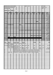
If you do not have access to the statistics toolbox you can use the function erf(x),which gives the error functionerf(x) = √ 2 ∫ xe −t2 dt πA comparison with F (x) suggests that the calculations above with x = 1.5, µ = 2 andσ = 0.7 can be made as>> (erf((1.5-2)/(0.7*sqrt(2)))+1)/2ans =0.2375Again, if you need to carry out similar calculations several times, you can create the filenormcdf.m in your working directory with the contentfunction y=normcdf(x,m,s)for i=1:length(x)y(i)=(erf((x(i)-m)/(s*sqrt(2)))+1)/2;end02 Exercises2.1 Cox-Ross-Rubinstein FormulaeIn the first exercise you are going to use historical data from the file histprices.txt on thecourse’s homepage again to price options on stock using Cox-Ross-Rubinstein Formulae.Import the file to Matlab in the same way as in the previous assignment and calculate thelogarithmic returns as>> k=log(data(2:251,:)./data(1:250,:));and choose one of the stock, for example by assigning an integer between 1 and 25 to thevariable stock.To be able to determine the price of an option on this stock we have to first define abinomial tree model for the price of one share of the stock. One way to determine u andd is to use the representation (3.7) in Section 3.3.2 in the textbook [2] and first estimatethe drift m and volatility σ as>> m=250*mean(k(:,stock));>> s=sqrt(250*var(k(:,stock)));4

Note that τ = 1/250 in this case since there were 250 trading days during the year.Assume that the risk-free interest rate is constant and 10 % during this period, whichgives the daily rate r = 0.10/250, and that the exercise price X of an option with exercisetime one year is determined asX = S(0)(1 + 0.10)i.e. that the stock is assumed to increase according to the risk-free interest rate during theyear.a. Determine the price of a European call option on your chosen stock at September1st, 2006 with exercise time one year and exercise price X.b. Calculate the value of the option after three, six and nine months. (Assume that thetrading days are evenly distributed over the year.)c. Determine the price of a European put option on your chosen stock at September1st, 2006 with exercise time one year and exercise price X.d. Calculate the value of the option after three, six and nine months.e. What happens to the initial prices if the interest rate drops to 5 % while X isunchanged?f. What happens to the initial prices if the volatility is doubled?(In reality, future prices of the stock are of course unknown when the price of the optionis determined. Usually, parameters are estimated from historical data from the time pointwhen the option is issued and backwards and then the value of the option is calculated asfuture stock prices become available. The method in this assignment is therefore circularand produces better results than it should, but the purpose of the exercise is to give practicein using the Cox-Ross-Rubinstein Formulae so we allow this simplification.)2.2 Black-Scholes FormulaeIn this exercise you are going to carry out the same calculations as in the previous exercisebut with the Black-Scholes formulae instead. These formulae are based on the geometricBrownian motionS(t) = S(0) exp(mt + σW (t))where W (t) is a Brownian motion and the drift m and volatility σ are the same as before.Assume the same constant risk-free interest rate r and exercise price X as before and carryout the exercisesa. Determine the price of a European call option on your chosen stock at September1st, 2006 with exercise time one year and exercise price X.5

. Calculate the value of the option after three, six and nine months. (Assume that thetrading days are evenly distributed over the year.)c. Determine the price of a European put option on your chosen stock at September1st, 2006 with exercise time one year and exercise price X.d. Calculate the value of the option after three, six and nine months.e. What happens to the initial prices if the interest rate drops to 5 % while X isunchanged?f. What happens to the initial prices if the volatility is doubled?g. Compare the results with the first exercise. How large is the difference?3 Written reportSolutions to all exercises must be presented in a structured report with a title sheet wherethe name of the course, the number of the assignment and your names clearly should beincluded. Hand written reports will not be accepted.Formulate your answers clearly and motivate all your conclusions exhaustively. Youare welcome to include or append some illustrative figures, but not too many and clearlydescribe in the text what conclusions you draw from each figure.References[1] Björkström, Anders (2002): Grundläggande Matlab-träning, Matematiska institutionen,Stockholms universitet.www.math.su.se/matstat/und/proci/pdf/matlabinstru.pdf[2] Capiński, Marek & Zastawniak, Tomasz (2003): Mathematics for Finance – An Introductionto Financial Engineering, Springer Verlag, London.[3] Holtsberg, Anders (2000): Introduktion till Matlab och Maple, Matematikcentrum,Lunds tekniska högskola.www.maths.lth.se/matstat/kurser/fms120/mlabintr.pdf[4] Moler, Clive (2004): Numerical Computing with MATLAB, MathWorks.www.mathworks.com/moler/chapters.html[5] Pärt-Enander, Eva & Sjöberg, Anders (2003): Användarhandledning för Matlab, Institutionenför informationsteknologi, Uppsala universitet.www.it.uu.se/edu/bookshelf/matlab/?lang=sv6