Transient Thermal Analysis of a Fin

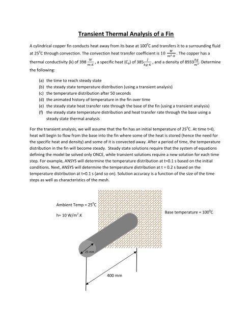
Transient Thermal Analysis of a FinA cylindrical copper fin conducts heat away from its base at 100 0 C and transfers it to a surrounding fluidat 25 0 C through convection. The convection heat transfer coefficient is 10 . The copper has a·thermal conductivity (k) of 398 , a specific heat (C p) of 385 , and a density of 8933· · . Determinethe following:(a) the time to reach steady state(b) the steady state temperature distribution (using a transient analysis)(c) the temperature distribution after 50 seconds(d) the animated history of temperature in the fin over time(e) the steady state heat transfer rate through the base of the fin (using a transient analysis)(f) the steady state temperature distribution and heat transfer rate through the base using asteady state thermal analysisFor the transient analysis, we will assume that the fin has an initial temperature of 25 0 C. At time t=0,heat will begin to flow from the base into the fin where some of the heat is stored (hence the need forthe specific heat and density) and some of it is convected away. After a period of time, the temperaturedistribution in the fin will become steady. Steady state solutions require that the system of equationsdefining the model be solved only ONCE, while transient solutions require a new solution for each timestep. For example, ANSYS will determine the temperature distribution at t=0.1 s based on the initialconditions. Next, ANSYS will determine the temperature distribution at t = 0.2 s based on thetemperature distribution at t=0.1 s (and so on). Solution accuracy is a function of the size of the timesteps as well as characteristics of the mesh.Ambient Temp = 25 0 Ch= 10 W/m 2 .KBase temperature = 100 0 C25 mm400 mm

TRANSIENT SOLUTIONBuild Model:1. Preprocessor >Element type > Add/Edit/Delete > (Add) > Thermal Mass > Solid > ( Solid 87) > OK(this 10 node tetrahedral element works well for the curved edges of the fin)2. Preprocessor > Material properties > Material models > Thermal >Enter Conductivity > Isotropic > KXX = 398, Specific heat C = 385, Density DENS = 89333. Preprocessor >Modeling > Create > Volumes > Cylinder > Solid cylinder > WP X = 0, WP Y = 0,Radius = 0.0125, Depth = 0.4 (use PlotCtrls to view an isometric of the cylinder)4. Preprocessor > Meshing > Mesh tool > Turn onsmart size to 4 > Mesh > Volumes > Mesh>(Pick the body) > OKDefine Loads, Time Stepping Options, Output Options & Solve:5. Solution > Analysis Type > New Analysis > Transient > OK > Full > OK6. Solution > Define Loads > Apply > Thermal > Temperature > On Areas > (pick base of fin) > TEMP100 > OK7. Solution > Define Loads > Apply > Thermal > Convection > On Areas > (pick all of the areasexcept for the base – there are 3 – just click 3 times near the tip of the fin) > Film Coefficient =10, Bulk Temperature = 25 > OK8. Solution > Define Loads > Apply > Initial Condit’n > Define > Pick All > Lab = TEMP, VALUE = 25(ANSYS will remember the base temperature and the convection conditions you entered for the steadystate solution, so you don’t have to re‐enter them. You can use the “List” tool to view these conditions)9. Solution > Load Step Opts > Time/Frequenc > Time‐Time Step > Set TIME = 10000 (at the top),KBC = stepped, AUTOTS = Prog Chosen, Minimum time step size = 0.01, maximum time step size= 200 > OK (We will let the ANSYS take charge of choosing the appropriate time step, limiting the timestep to 200s)10. Solution > Load Step Opts > Output Ctrls > DB/Results File > FREQ = every substep > OK (settingthis option will allow us to see contour plots and obtain other results at any time step between t = 0 and t= 10,000s)11. Solution > Solve > Current LS > OKIt will take the model a while to run since it will require at least 50 time steps (max time = 10000 dividedby maximum time step = 200)

Time History Post Processing:12. Timehist postproc > DefineVariables > Add > Nodal DOFResult > OK > Select a noderandomly at the middle ofthe end of the fin > OK >NVAR = 2, DOF solution=Temp >OK13. Timehist Postproc > GraphVariables > NVAR1 = 2 > OK(This gives the variation oftemperature with respect totime at that node. Notice thatsteady state conditions arereached at about 3000s, with avalue of 80 degrees C at the tip)14. Timehist Postproc > List Variables >NVAR1 = 2 > OK (this lists the temperature as a function of timeat the tip, as shown below)TIMETEMP1.0000 25.00001.4996 25.00001.8532 25.00002.2069 25.00003.1585 25.00004.6611 25.00006.9792 25.000010.514 25.000015.871 25.000223.959 25.003836.129 25.039354.375 25.249881.646 26.0619122.92 28.2982189.89 33.2269310.34 42.2421499.94 53.3552699.94 61.7352899.94 67.57641099.9 71.61411299.9 74.39721499.9 76.31371699.9 77.63301899.9 78.54122099.9 79.16632299.9 79.59652499.9 79.89272699.9 80.09652899.9 80.23683099.9 80.33343299.9 80.39983499.9 80.4456TIMETEMP3699.9 80.47713899.9 80.49874099.9 80.51364299.9 80.52394499.9 80.53104699.9 80.53584899.9 80.53925099.9 80.54155299.9 80.54315499.9 80.54425699.9 80.54495899.9 80.54546099.9 80.54586299.9 80.54606499.9 80.54626699.9 80.54636899.9 80.54647099.9 80.54657299.9 80.54657499.9 80.54657699.9 80.54657899.9 80.54668099.9 80.54668299.9 80.54668499.9 80.54668699.9 80.54668899.9 80.54669099.9 80.54669299.9 80.54669499.9 80.54669699.9 80.54669899.9 80.546610000. 80.5466

General Post Processing:15. General Postproc > Read Results> Last Set16. General Postproc > Plot Results >Contour Plot > Nodal Solution >DOF Solution > NodalTemperature > OK (this is thetemperature distribution at 10,000sor the steady state temperatures)17. General Postproc > Read Results> By Time/Freq > Enter TIME = 50> OK18. General Postproc > Plot Results >Contour Plot > Nodal Solution >DOF Solution > NodalTemperature > OK (this is thetemperature distribution at 50s)

19. General Postproc > Readresults > By time/freq >Enter TIME = 180 > OK20. General Postproc > Plotresults > Contour plot >Nodal solution > DOFsolution > Nodaltemperature > OK(Notice the changes in thetemperature distributionrelative to thetemperatures at 50s.Higher temperatures aremoving further down therod.)21. PlotCtrls > Animate > Over Time > click on Time Range and enter 0 for a minimum time and 3000for a maximum time > OK (This will show an animation of temperature with time. You can varysettings.)22. General Postproc > Read Results > Last Set23. General Postproc > List Results > Reaction Solu > Heat flow > OK (scroll to the bottom of the list tosee that the steady state total heat flow through the base of the fin is 19.7 W)STEADY STATE SOLUTIONThe transient solution must converge to the steady state solution. It is important to check the transientsolution using a steady state analysis. The steady state model does not rely on the heat capacity,density, or initial conditions.Build Model:1. Preprocessor >Element type > Add/Edit/Delete > (Add) > Thermal Mass > Solid > ( Solid 87) > OK(this 10 node tetrahedral element works well for the curved edges of the fin)2. Preprocessor > Material properties > Material models > Thermal >Enter Conductivity > Isotropic > KXX = 3983. Preprocessor >Modeling > Create > Volumes > Cylinder > Solid cylinder > WP X = 0, WP Y = 0,Radius = 0.0125, Depth = 0.4 (use PlotCtrls to view an isometric of the cylinder)