stress analysis - Mechanical and Mechatronics Engineering ...

STRESS ANALYSIS and FATIGUE of welded structuresSTRESS ANALYSIS and FATIGUE of weldedstructuresA. Chattopadhyay, G. Glinka, M. El-Zein, J. Qianand R. Formasanalyses of weldments require detailed knowledge of the stress fields in critical regions. The stressinformation is subsequently used for finding high local stresses where fatigue cracks may initiate and for calculatingstress intensity factors and fatigue crack growth. The method proposed enables the determination ofthe stress concentration and the stress distribution in the weld toe region using a special shell finite elementmodelling technique. The procedure consists of a set of rules concerning the development of the finite elementmesh necessary to capture the bending and membrane structural stresses. The structural stress dataobtained from the shell finite element analysis and relevant stress concentration factors are subsequentlyused to determine the peak stress and the non-linear through-thickness stress distributions. The peak stressthe weld toe is subsequently used for the determination of fatigue crack initiation life. The stress distributionand the weight function method are used for the determination of stress intensity factors and for the analysisof subsequent fatigue crack growth.ABSTRACTFatigueIIW-Thesaurus keywords: Structural analysis; Stress distribution; Finite element analysis.21 IntroductionFatigue processes originate at stress concentration points,such as the weld toe in weldments. Both the fatigue crackinitiation and propagation stages are controlled by themagnitude and the distribution of stresses in the potentialcrack plane. The peak stresses at the weld toe can becalculated using stress concentration factors, available inthe literature, and appropriate reference stresses. Thesestress concentration factors are unique for given geometryand mode of loading. However, weldments are oftensubjected to multiple loading modes, and therefore it isnot easy to define a unique nominal or reference stress.For this reason, the use of classical stress concentrationfactors is limited to simple geometry and load configurationsfor which they were derived. This problem can beresolved by using the hot spot or structural stress, σ hsconceptapplied initially in the offshore structures industry [1].If the stress concentration factors, based on the hot spotstress, σ hsas the reference (or nominal stress), are knownthen the shell or coarse 3D finite element mesh models[2] can be used to determine only the hot spot stress atthe weld toe and subsequently to determine the peakstress by using appropriate stress concentration factors.Unfortunately, the hot spot stress based stress concentrationsfactors vary for the same geometry dependingon the type of loading, i.e. such stress concentration factorsare not unique for a given geometry. This is a seriousdrawback if various multiple loads are applied to the sameweldment or welded structures.The purpose of the method discussed below is to find suchan approach that would require only stress concentrationfactors independent of the load configuration and appropriatereference stresses to be used. The only parametersneeded for estimating the stress peak and the stressdistribution induced by any combination of loads are onlythe geometrically unique stress concentration factors andappropriate reference or nominal stresses.2 The nature of the stressesin the weld toe regionThe stress state at the weld toe is multi-axial in nature. Butthe plate surface is usually free of stresses, and thereforethe stress state at the weld toe is in general reduced toone non-zero shear and two in-plane normal stress components(Figure 1). Due to stress concentration at theweld toe the stress component, σ yynormal to the weldtoe line is the largest in magnitude and it is predominantlyresponsible for the fatigue damage accumulation in thisregion. Therefore, it is sufficient in practice to considerfor the fatigue analysis of welded joints only the stresscomponent, i.e. its magnitude and distribution across theplate thickness.Doc. IIW-2201, recommended for publication by Commission XIII “Fatigue of Welded Components and Structure.”1106_0037_WELDING_7_8_2011.indd 2 14/06/11 10:35:01

STRESS ANALYSIS and FATIGUE of welded structuresthe reference point A must coincide with thephysical position of the weld toe. Thus stressesat the reference point A are the same as thenodal stresses and they can be extractedwithout any interpolation or additional postprocessing.d. The dimension ‘z’ of the first two rows of elementsadjacent to the intersection of platemid-thickness planes is dictated by the smallestelement in the region, i.e. it should not begreater than half of the weld leg length ‘h/2’. Itmeans that the first and the second row of elementsin the main plate [Figure 8 b)] have thedimension of [(h/4 + t p/4) × h/2]. The first tworows of elements in the attachment countedfrom the mid-plane intersection should havethe size of [(h/4 + t/4) × h/2]. The elementsin the third row are (h/2 × h/2) in size. Thespacing in the ‘z’ direction might need to besmaller than half of the weld leg length ‘h/2’while modelling corners of non-circular tubesor weld ends around gusset plates.5.1 Determination of the peak stressat the weld toeIn order to determine the peak stress σ peakat the weld toeit is necessary to determine the membrane m hs and bending b hs stress from the shell finite element model usingEquations (8-9). Then the stress concentration factorsmbKths , and Kths , for tension and bending need to be calculatedfrom Equations (4-5) or (6-7) by using actual dimensionsof the weld. The peak stress σ peakcan be finally calculatedfrom Equation (1).The knowledge of the linear elastic peak stress σ peakenables subsequently the assessment of the fatiguecrack initiation life by applying the local strain-life methodwidely used in the automotive industry [9-12].5.2 Determination of the through-thicknessstress distributionBecause welded structures are known as having highstress concentration at weld toes and roots the fatiguecrack initiation period might be relatively short and thereforefatigue life assessment based on the fatigue crackgrowth analysis is often required. In order to carry out ameaningful fatigue crack growth analysis appropriatestress intensity factor solutions are needed. Because ofwide variety of possible configurations of the global jointgeometry, the weld geometry, the crack geometry andloading reliable ready-made stress intensity solutions areseldom available. Therefore the weight function method(discussed later) seems to be a convenient and efficientsolution but the through-thickness stress distribution in theprospective crack plane must be known in such a case.It has been found that the same information, i.e. themembrane m hs and bending b hs hot spot stresses andmbassociated stress concentration factors Kths , and Kths , aresufficient for the determination of the through-thicknessdistribution denoted as distribution B in Figure 2 b).The stress distribution, needed for the stress intensity factorK calculation, can be determined by using universalstress distributions proposed by Monahan [13]. Both equationsshown below were derived for the through-thicknessstress distribution in a T-butt weldment (Figure 5) but theycan also be applied over half of the thickness in the caseof cruciform weldments (i.e. for a weldment with symmetricwelds located on both side of the plate as shown inFigure 6).For pure tension loading the through-thickness stressdistribution can be sufficiently accurate approximated byEquation (10).1 3m mKths, 1 2 1 1 2mhs x x 1 x 2 2 r 2 2 r 2G(10)m wherexGm1for 0.3rEmTm0.94 exGm0.06 for 0.31.13 0.8 EmT1ETem rm mq0.18 rEm1.05 tq = −0.12Θ −0.62Tmx r 0.3t tFor pure bending load Equation (11) is recommended:1 3 x b b1 2Kths, hs 1 2 1 1 2bx x t x (11)2 2 r 2 2 r 2 Gb wherexGb1for 0.4rETb b0.93 exGb0.07 for 0.41.23 0.6 ETb b1ETerrEb 0.9 tx rTb 0.4t tb 0.0825 0.0026 bEquations (10-11) can be used to predict through-thicknessstress distributions near fillet welds joining plates,tubes and other structural elements providing that parametersΘ, r/t, and x are within the following limits: 1 r 1 and and 0 x t (12)6 3 50 t 15If both membrane and bending stresses are present theresultant through-thickness stress distribution can beobtained by superposition of Equations (10) and (11).707N° 08 2011 Vol. 55 WELDING IN THE WORLD Peer-reviewed Section1106_0037_WELDING_7_8_2011.indd 7 14/06/11 10:35:09

STRESS ANALYSIS and FATIGUE of welded structures8 x m m b b1 2m b Kt hs 1 Kt hs t x xx 2 2 Gm2 2 Gb1 3 x 1 2 1 x 1 2 (13) r 2 2 r 2Appropriate weight functions [14-15] and the stressdistribution (13) make it possible to determine stressintensity factors and to subsequently simulate the fatiguecrack growth in any welded structure without the labourand time consuming extensive FE numerical analyses ofcracked bodies. In addition the method is self-consistentand does not require making any arbitrary adjustments.6 Fatigue crack initiation analysisThe maximum of the peak stress σ peak,maxand the peakstress range Δσ peakat the weld toe can be subsequentlyused for the calculation of the actual stresses and elasticplasticstrains at the weld toe. The most common methodis the use of the Neuber [9] or the ESED [10] method andthe material cyclic stress-strain curve in the form of theRamberg-Osgood expression. 2,maxamaxpeak a amaxmaxE – the Neuber rule (14)1a a 'maxnmax' E K – the material Ramberg-Osgood stress-strain curve (15)In order to Calculate the elastic-plastic strain range andcorresponding stress range the same Neuber rule associatedwith the stress-strain curve expanded by factor of 2can be used. 2peak a aE – the Neuber rule (16)1a an''a 2 E 2 K – the expanded material stressstraincurve (17)Because it is known that the Neuber rule has the tendencyof overestimating the local elastic-plastic strainsand stresses at high stress concentration factors theEquivalent Strain Energy Density (ESED) method can beused in the form of analogous set of equations for obtainingthe maximum elastic-plastic strain and stress at theweld toe.2 1a2' a apeak namax,max max max max'' – the ESED rule2E 2E n 1 K (18)1a a 'maxnmax' E K – the material Ramberg-Osgoodstress-strain curve (19)The same ESED rule but combined with the expanded byfactor of 2 stress-strain curve is applied for calculating theelastic-plastic strain and stress range.2 peak 21a a a2 n''' 2E 2E n 1 2K1a an''a 2 E 2 K – the ESED rule(20)– the expanded material stressstraincurve (21)aThe actual maximum stress at the weld toe and themaxactual strain range Δε a obtained from Equations (14-17)or (18-21) formulate the base for calculating the numberof cycles, N i, to initiate a fatigue crack at the weld toe.The basic fatigue material property is the strain-life equationproposed [11] by Manson and Coffin.'b ' cf2Ni f 2Ni(22)2EIn order to account for the mean stress effect or the existenceof residual stresses the SWT [12] fatigue damageparameter can be used in association with the Manson-Coffin curve.'2f 2 b ' 'bc Nf ff Nfaa max 2 2(23)2 EUnfortunately, the strain-life method does not specifywhat crack size is associated with the end of the initiationperiod therefore an engineering definition needs tobe adopted. Based on author’s experience a semi-circularcrack of the initial depth of a i= 0.5-0.8 mm seems to be areasonable good assumption.It is worth noting that there are several fatigue softwarepackages for which the local elastic stress σ peakandmaterial curves (13) and (19) are the standard input datafor automatic fatigue crack initiation life assessment.Therefore, the method described above can be associatedwith any available computer fatigue software package.7 The fatigue crack growth analysisThe fatigue crack growth period is often thought to berepresenting almost the entire fatigue life of weldmentsbecause it is believed that the fatigue crack initiationperiod in welded joints is relatively short. The authorsexperience is that the ratio of the fatigue crack initiationlife to the length of the fatigue crack growth period variesdepending on the load and weld geometrical factorsand its relative contribution to the total fatigue life of aweldment increases in with the decrease of the appliedcyclic load and the increase of the total life. Thereforegood assessments of both the fatigue crack initiation andpropagation period are necessary for reasonably accurateestimation of fatigue lives of weldments subjected tocyclic loading histories.1106_0037_WELDING_7_8_2011.indd 8 14/06/11 10:35:10

STRESS ANALYSIS and FATIGUE of welded structuresThe first and the most popular expression characterizingmaterial properties from the point of view of the materialresistance to fatigue crack growth is the Paris [16]equation.da C K mdN (24)Unfortunately, the Paris equation in its original form (24)does not account for the effect of the stress ratio R orthe mean stress. Therefore the recently proposed [17, 18]Equation (25) is gaining popularity.dadNwhere1p pCKmax K(25)C, p, m and γ are material constants, K maxis the maximumstress intensity factor and ΔK is the stress intensity range.In the case of pulsating constant amplitude stress history(R = 0) Equation (25) takes the well-known form of theParis equation.The fatigue crack propagation life is obtained by analyticalor numerical integration of the fatigue crack growthequation.af da daNpor N C K C K K aimp1p p max afai(26)However, in order to Integrate any fatigue crack growthrate expression available in the literature the stress intensityfactors K maxand ΔK need to be determined.7.1 Application of the weight functionmethod for efficient determinationof stress intensity factorsIn the case of simple geometry and load configurationslike the edge or semi-elliptical surface crack in a platesubjected to pure bending or tension load ready-madestress intensity factor expressions can be found [19] inHandbooks of Stress Intensity Factors. Unfortunately,there are no ready-made solutions for cracks in weldedstructures except for a few crack configurations in simplewelded joints. Therefore the weight function technique[14, 15] was employed in order to determine stress intensityfactors for cracks in real welded structures.The weight function can be understood as the stressintensity factor (Figure 9) induced by the simplest loadconfiguration, i.e. a pair of unit splitting forces F attachedto the crack surface.There are many expressions for various weight functions butit is possible [15] to write them in one general form (27).12P 2F x mx, aKA 1M112ax a 3(27) x x 2M21 M31 a a Parameters M 1, M 2and M 3depend on the crack geometryand they have been derived already [15] for a variety ofcracks. The M iparameters for a single edge and surfacesemi-elliptical crack are given in reference [15] and listedin the Appendix.If the weight function is known, the stress intensity factorK can be calculated by integrating the product of thestress distribution, σ (x), in the prospective crack plane andthe weight function m(x,a): ( x )Aa , (28)K x m x a dx0Figure 9 – Notation for the weight functionThus, the calculation of stress intensity factors by theweight function method for any crack, including cracks inweldments, requires the knowledge of the stress distribution,σ (x), in the prospective crack plane in the un-crackedbody [Figure 10 a)] and then the stress distribution shouldbe virtually applied to the crack surfaces [Figure 10 b)].Figure 10 – The use of the weight functionfor an edge crack in plate for calculating the SIFfor a crack in a T-butt weldment907N° 08 2011 Vol. 55 WELDING IN THE WORLD Peer-reviewed Section1106_0037_WELDING_7_8_2011.indd 9 14/06/11 10:35:11

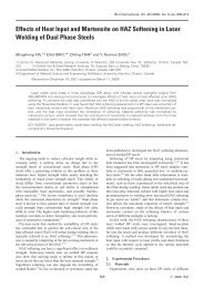
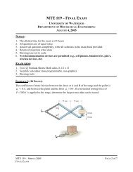
STRESS ANALYSIS and FATIGUE of welded structuresFinally the product of the stress distribution σ (x) and theweight function m(x,a) needs to be integrated over theentire crack surface area [see Equation (28)]. It is to notethat the stress analysis needs to be carried out only onceand for an un-cracked body [Figure 10 a)].The stress intensity factor calculations can be repeatedafter each crack increment induced by subsequent loadcycles so the stress intensity factor is calculated for theinstantaneous (actual) crack size and geometry. Such amethod enables simulation of the crack growth and theevolution of the crack shape in the case of 2D planarcracks.108 Stress and fatigue analysisof a tubular welded sectionsubjected to constant amplitudefully reversed torsionand bending loadsSeveral welded structures and welded joints were studiedexperimentally and numerically in order to verify thevalidity of the proposed methodology. The welded structureshown in Figure 11, subjected to torsion and bendingload, was chosen as an example for illustrating thestepwise procedure. The overall geometry of the weldedjoint fixed in the testing rig is also shown in Figure 11.Dimensions of selected welded tubular profiles were4 x 4 x 23.625 in and 2 x 6 x 14.313 in and the wallthicknesses were equal to 0.312 in. The geometricalconstrains of the fixture and the location of the appliedload is shown in Figure 12. The welded tubular profileswere made of A22-H steel (ASTM A500 Cold FormedSteel for Structural Tubing) used often in the constructionand earth moving machinery. The manual Flux CordArc Welding method was used to manufacture a seriesof specimens. The welding parameters were typical formanual welding aimed at the maximum weld penetrationFigure 11 – The tubular welded joint subjected to torsionand bending load in the testing rigFigure 12 – Solid model of the welded joint- configurationof support points and the location of the loading forceand maximum uniformity of weld geometry along its entirelength. The average weld dimensions obtained from thewelding process were (see Figure 5):t = 0.312 in, t p= 3 x 0.312 in, h = 0.312 in, h p= 0.312 in,Θ = 45°, r = 0.0312 inThe specimens were tested at two different cyclic loadlevels of ± 3 000 lb and ± 4 000 lb applied at the freeend of the large square profile (Figure 12). The bottombase plate of the fixture was held by six screws. In orderto assess anticipated scatter of experimental fatigue livesseven specimens were tested at each load level.8.1 The shell FE stress analysisThe shell model of the analysed welded tubular joint ispresented in Figure 13. The overall stress field obtainedfrom the FE analysis of the entire structure is also showngraphically in Figure 13. Three high stress locations wereidentified with the highest stresses found at Location 1.Therefore detail analysis of stresses at Location 1 wasundertaken. The exact location of the maximum stresswas found in the region around the ending edge of therectangular tube. The stresses of interest were thosefound at the reference point shown in Figure 14 of theshell model. The location of the reference point was coincidingas usual with the physical position of the weld toein the actual weld joint. The distance between the referencepoint and the tube wall mid-planes intersection pointin the shell FE model was equal to:t p0.312h 0.312 0.468 in2 2The shell stresses 1 hs and 2 hs on opposite sides of thetube wall (see Figure 7), obtained from the shell FEmodel, were used for the determination of the membraneand bending [Equations (8-9)] hot spot stresses, m hs and hs, b respectively. The peak stress at the weld toe,σ peak, was determined from Equation (1). The through-1106_0037_WELDING_7_8_2011.indd 10 14/06/11 10:35:12

STRESS ANALYSIS and FATIGUE of welded structuresFigure 14 – Details of the shell FE model and the locationof the reference point for determining the hot spot stressFigure 13 – The shell finite element model of the weldedjoint showing overall stress distribution with three distinctregions of high stressesthickness stress distribution, σ (x), was calculated usingEquations (10-11,13).The shell stresses induced by the unit load of P = 1.0 lbon the two sides of the tube wall and calculated using theshell FE data were:1hs= 8.25 psi and = −3.05 psi2hs11Therefore the hot spot stresses determined according toEquations (8) and (9) were:1 2 8.25 3.05m hs hshs 2.6 psi2 21 2 8.25 3.05b hs hshs 5.65 psi2 2mbThe stress concentration factors Kths , and Kths , obtainedfrom Equations (4) and (5) for geometrical dimensionst = 0.312 in, t p= 3t = 0.936 in, h = 0.312 in, h p= 0.312 in,mbr = 0.0312 in and Θ = 45°, were Kths , = 1.784 and Kths ,= 2.203. The hot spot stresses corresponding to the unitload P = 1 lb and the stress concentration factors inputtedinto Equation (1) resulted in the determination of thepeak stress at the weld toe.σ peak= m mhs ⋅ Kths , + b ⋅ bhsKths , = 2.6 x 1.784 = 5.65 x 2.203= 17.089 psi. In order to determine stresses correspondingto the actual load P = 3 000 lb or 40 000 lb the stressσ peak= 17.089 psi was scaled by the factor of 3000 or4000 depending on the applied load magnitude.The through-thickness stress distribution σ (x) wasobtained using the universal Equations (10-11 and 13)and geometrical parameters, hot spot stresses and stressconcentration factors listed above. The through-thicknessstress distribution induced by the applied external forceP = 3 000 lb is shown in Figure 15.In order to verify the accuracy of the shell FE basedmethod a very detail 3D FE stress analysis was alsoFigure 15 – Through-thickness stress distributionat Loc. 1 induced by the unit load P = 1 lbcarried out for the same welded joint. The through-thicknessstress distribution obtained from the 3D fine meshFE model (Figure 16) is also shown in Figure 15. It can benoted that the stress distribution obtained from the coarsemesh shell FE model and Monahan’s equations coincidevery well with the stress distribution obtained from thevery detail and fine 3D FE mesh model of the same jointshowing good accuracy of the proposed methodology.Similar results were obtained for a variety of other weldedstructures.In addition to the FE calculations of the through-thicknessstress distribution induced by the applied load P(Figure 12) several X-ray measurements of weldingresidual stresses were carried out on a few full scalewelded joints. Based on the X-ray measurements and theforce and bending moment equilibrium requirements theapproximate through-thickness residual stress distributionat the hot spot Location 1 has been estimated and itis shown in Figure 17. The actual maximum residual stressdistribution measured in the closed proximity of the referencepoint (Figures 11 and 13) in as-welded joints wasσ r0= 45 ksi.07N° 08 2011 Vol. 55 WELDING IN THE WORLD Peer-reviewed Section1106_0037_WELDING_7_8_2011.indd 11 14/06/11 10:35:18

STRESS ANALYSIS and FATIGUE of welded structuresFigure 16 – Details of the 3D fine mesh FE modelof the critical locationFigure 17 – Through-thickness residual stress distributionat Location 1129 Experimental and theoreticalfatigue analysesThe fatigue life was predicted as a sum of the crack initiationlife (the strain-life method) and crack propagation life(the fracture mechanics approach). In order to comparepredicted lives with the experimental data, two series oftests were carried out. The first one was conducted at thefully reversed cyclic load of ± 3 000 lb and the other at± 4 000 lb.All experiments were carried out under the load controlconditions and the crack length 2c, visible on the surface,was measured versus the number of applied load cycles.Optical measurements with the aid of magnifying glasswere carried out throughout all tests.The peak stresses at the weld toe and the throughthicknessstress distributions induced by the appliedloads were obtained by scaling the stress distribution ofFigure 12, obtained for the unit load P = 1 lb, by factor3000 and 4000.9.1 Fatigue crack initiation life analysisof tested welded jointsThe fatigue crack initiation life was predicted using the inhouseFALIN fatigue software with implemented strain-lifefatigue live prediction procedure. The procedure is brieflydescribed in Section 6. The elastic-plastic stresses andstrains at the weld toe were calculated for each load cyclebased on the Ramberg-Osgood stress strain curve (13)and the Neuber Equation (12). These strains and stresseswere used in the Smith, Watson, and Topper (SWT) strainlifeEquation (20) for calculating the fatigue life to crackinitiation. The fatigue crack initiation life calculations werebased on the material properties listed below.The monotonic and fatigue (cyclic) properties of theA22-H steel material are listed in Table 1 and Table 2respectively.The resultant amplitude of the fully reversed (R = -1) cyclicstress at the weld toe Location 1 obtained from the linearelastic analysis was σ a= 51.27 ksi and σ a= 68.36 ksi forthe load 3 000 lb and 4 000 lb respectively.The assessed fatigue crack initiation lives, N i, are listedin Tables 3 and 4. Unfortunately comparison of calculatedfatigue crack initiation lives with experimental datais not very meaningful because the method itself doesnot specify what crack size corresponds to the end ofrather vaguely defined crack initiation period. Thereforean engineering definition of the crack initiation size, basedon experimental data, needs to be employed. The experimentaldata analysed by the authors up to date indicatedthat the predicted fatigue crack initiation lives coincidedmost often with lives (number of cycles) needed for thecreation at the weld toe of semi-elliptical cracks of deptha i= 0.02 in with the aspect ratio a i /c i = 0.286.Table 2 – The cyclic and fatigue propertiesof the A22-H steel materialFatigue strength coefficient (σ’ f) [ksi] 169.98Fatigue strength exponent (b) -0.12Fatigue ductility coefficient(ε’ f) 0.648Fatigue ductility exponent (c) -0.543Cyclic strength coefficient (K’) [ksi] 155.2Cyclic strain hardening exponent (n’) 0.187Ultimate strength (S u)[ksi]Table 1 – Monotonic mechanical properties of the A22-H steel materialYield strength (S y)[ksi]Elastic modulus (E)[ksi]79.0 68.89 29 9381106_0037_WELDING_7_8_2011.indd 12 14/06/11 10:35:32

STRESS ANALYSIS and FATIGUE of welded structuresThe fatigue crack analyses were carried out for two loadlevels (3 000 lb and 4 000 lb) with and without residualstresses. The residual stress was combined with the cyclicstress induced by the applied load by including it [20, 21]into the Neuber or ESED equation in such a way that onlythe actual maximum elastic-plastic strain and stresses atthe weld toe were affected. 2,max 0peak r a amaxmaxE – the Neuber rule (29)2 1a2' a apeak r n,max 0 max max max'' – the ESED rule2E 2E n 1 K (30)The magnitudes of the elastic-plastic strain and stressranges were not affected by the static residual stress andthey can be determined according to Equations (16-17)or (20-21).It is noticeable (see Tables 3 and 4) that the residualstress had profound effect on the fatigue crack initiationlife. The analysis indicates that the tensile residual stressat the weld toe may decrease the fatigue crack initiationlife by approximately factor of 3.9.2 The fatigue crack growth analysisThe second part of the fatigue life assessment was devotedto the fracture mechanics based analysis of fatigue crackgrowth. The fatigue crack growth analysis was carried outusing the in-house FALPR software package enablingthe calculation of stress intensity factors based on theweight function method and subsequent cycle by cyclefatigue crack growth increments. The observed fatiguecracks were semi-elliptical in shape (Figure A2) with initialdimensions of a i= 0.02 in and 2c i= 0.14 in, i.e. the initialaspect ratio was a/c = 0.238. The semi-elliptical surfacecrack in a finite thickness plate was assumed to be theappropriate model for fatigue crack growth simulations.The stress intensity factors for the actual crack shape(a/c) and depth, a, were calculated using the weight functiongiven by Equations (A1-A50). Stress intensity factorsand crack increments at points A and B (Figure A2) weresimultaneously calculated on cycle by cycle basis. As aresult the crack growth and the crack shape evolutionwere simultaneously simulated.The through-thickness stress distribution induced by theexternal load shown in Figure 15 and the residual stressof Figure 17 were used for the determination of stressintensity factors. The crack increments induced by subsequentload cycles were calculated by using the Parisfatigue crack growth Equation (24) valid for R = 0.5 withparameters:m = 3.02 and C = 2.9736 x 10 -10 for ΔK in [ksi√in] andda/dN in [in/cycle].The threshold stress intensity range and the fracturetoughness for this material were:ΔK th= 3.19 ksi√in at R = 0 and K C= 72.81 ksi√in.It should be noted that the crack was not growing with thesame rate in all directions. Therefore crack increments atthe deepest point A and those on the surface (point BFigure A2) were determined separately for each cycle.The crack dimensions and the crack aspect ratio (a/c)were updated after each load cycle. The fatigue crackgrowth predictions were carried out first neglecting andsecondly including the residual stress effect.In order to account for the residual stress effect the methoddescribed in reference [21] and the modified Paris equationaccounting for the stress ratio R were used.da / dN = C (U ⋅ ΔK) m (31)The U parameter accounting for the stress ratio effect wasgiven by Kurihara [22] for a wide range of stress ratios inthe form of Equation (32)1U for 5.0 R0.51.5 R(32)U = 1 for R > 0.5First the maximum and minimum stress intensity factorsfor a given loading cycle were determined using the weightfunction Equation (A9) and Equation (A33) and the loadinduced stress distribution σ (x) shown in Figure 15.maxa0max , K x m x a dxmina0min , K x m x a dx(33)Then the stress intensity factor contributed by the residualstress σ r(x) shown in Figure 17 was also calculated usingthe same weight functions given by Equation (A9) andEquation (A33).ra r , (34)0K x m x a dxFinally all stress intensity factors were combined and theeffective stress ratio was determined.Kmin KrReffK K(35)maxrThe effective stress ratio enabled to determine the actualvalue of the U parameter in Equation (31) and calculatethe crack increment induced by analyzed loading cycle.This process was carried out simultaneously for bothpoints A and B (Figure A2) of the semi-elliptical surfacecrack.An example of the crack depth growth versus the numberof applied loading cycles (a vs. N), the evolution ofthe crack aspect ratio (a/c vs. N) and the evolution ofthe crack from its initial to the final shape are show inFigure 18. The experiments and fatigue crack calculationswere carried out until the crack reached approximate1307N° 08 2011 Vol. 55 WELDING IN THE WORLD Peer-reviewed Section1106_0037_WELDING_7_8_2011.indd 13 14/06/11 10:35:33

STRESS ANALYSIS and FATIGUE of welded structures14Figure 18 – Fatigue crack growth curve, a vs. N; evolutionof the crack aspect ratio a/c vs. N and evolutionof the crack shape; obtained for load 3 000 lb and σ r0= 0depth of a f= 0.14 in. The numerical analyses were carriedout using the following geometrical dimensions (seeFigure 5) of the weld:t = 0.312 in, t p= 3t = 0.936 in, h = 0.312 in, h p= 0.312 in,r = 0.0312 in and Θ = 45°.Statistical analysis was performed on large number (morethan 100 measurements) of measured real weld toeradii and weld angles and the most frequent values givenabove were used for the numerical analyses. All calculatedfatigue crack growth lives are summarized in Tables 3 and4. In addition fatigue crack lengths 2c versus number ofapplied load cycles N measured on seven specimens andthose calculated ones are shown in Figure 19.Summaries of predicted fatigue crack growth periods aregiven in Tables 3 and 4.The a/c vs. N curve shown in Figure 18 indicated thatthe crack was initially growing faster into the depth directionbut after reaching the aspect ratio of approximatelya/c = 0.5 it started growing faster along the weld toetending to the single edge crack geometry. This conclusionis supported by the actual shape of the final crack(Figure 20) after break-opening one of the specimens.Figure 19 – Experimental surface crack measurementsof the crack length ‘2c’ on seven specimens and predicted‘2c vs. N’ curves obtained under the cyclic load of ± 4 000 lbIt is clear that assuming constant aspect ratio for easierfatigue crack growth analysis may contribute to significanterror. Moreover, the surface crack measurements withoutany supporting theoretical crack growth simulations arenot sufficient for reliable estimation of the crack depth ‘a’.According to the data above the ratio of the crack initiationto the crack propagation life N i/ N p≤ 0.303 and thecrack initiation life to the total fatigue life N i/ N f≤ 0.233were rather low (and) indicating that majority of the fatiguelife of analysed weldment was spent on propagating theFigure 20 – The final shape of the fatigue crack initiatedat the weld toe around the edge of the rectangular tubeResidual stress [ksi]Table 3 – Summary of predicted fatigue lives under load P = 3 000 lbN i(Cycles)a i= 0.02 inN P(Cycles)a f= 0.14 inN i/N PN f(Cycles) N i/N fσ r0= 0 93 105 683 000 0.136 776 105 0.12σ r0= 45 27 939 92 000 0.303 119 939 0.233Residual stress [ksi]Table 4 – Summary of predicted fatigue lives under load P = 4 000 lbNi (Cycles)ai = 0.02 inNP (Cycles)af = 0.14 inNi/NP Nf (Cycles) Ni/Nfσ r0= 0 25 039 286 500 0.087 311 539 0.08σ r0= 45 10 602 49 975 0.212 60 577 0.1751106_0037_WELDING_7_8_2011.indd 14 14/06/11 10:35:34

STRESS ANALYSIS and FATIGUE of welded structures[12] Smith KN, Watson P, Topper TH.: A stress–strainfunction for the fatigue of metals, Journal of Materials,1970, vol. 5, no. 4, pp. 767-778.[13] Monahan C.C.: Early fatigue cracks growth at welds,Computational Mechanics Publications, Southampton UK,1995.[14] Bueckner H.F.: A novel principle for the computationof stress intensity factors, Zeitschrift fur AngewandteMathematik Und Mechanik, 1970, vol. 50, pp. 529-546.[15] Glinka G. and Shen G.: Universal features of weightfunctions for cracks in Mode I, Engineering FractureMechanics, 1991, vol. 40, no. 6, pp. 1135-1146.[16] Paris P.C. and Erdogan F.: A critical analysis of crackpropagation laws, Journal of Basic Engineering, 1963,no. D85, pp. 528-534.[17] Noroozi A.H., Glinka G. and Lambert S.: A twoparameter driving force for fatigue crack growth analysis,International Journal of Fatigue, 2005, vol. 27, no. 10-12,pp. 1277-1296.[18] Mikheevskiy S. and Glinka G.: Elastic–plastic fatiguecrack growth analysis under variable amplitude loadingspectra, International Journal of Fatigue, 2009, vol. 31,no. 11-12, pp. 1828-1836.[19] Murakami Y.: Stress intensity factors handbook,1987, vol. 2, Pergamon Press, Oxford.[20] Glinka G.: Residual stresses in fatigue and fracture:Theoretical analyses and experiments, Advances inSurface Treatments, vol. 4, A. Niku-Lari, Ed., InternationalJournal of Residual Stresses, 1987, pp. 413-454.[21] Glinka G.: Effect of residual stresses on fatiguecrack growth in steel weldments under constant and variableamplitude loading, Fracture Mechanics, ASTM STP677, C.W. Smith, Ed., American Society for Testing andMaterials, 1979, pp. 198-214.[22] Kurihara M., Katoh A. and Kwaahara M.: Analysis onfatigue crack growth rates under a wide range of stressratio, Journal of Pressure Vessel Technology, Transactionsof the ASME, May 1986, vol. 108, no. 2, pp. 209-213.161106_0037_WELDING_7_8_2011.indd 16 14/06/11 10:35:35

STRESS ANALYSIS and FATIGUE of welded structures11 Appendix - Selected one-dimensional (1D) weight functions for cracks in platesFigure A1 – Weight function notations for a single edge and central through crack in finite with plateSingle edge crack in a finite with plate (Figure A1, valid for 0 < a/t < 0.9)171 32 2F 2F x x xmx, a KA 1 M11 M21 M31 2 a x a a aaaaa 0.029207 0.213074 3.029553 5.901933 2.657820t t t tM1aaaaa 1.0+ 1.259723 0.048475 0.481250 0.526796 0.345012t t t t taaaa 0.451116 3.462425 1.078459 3.558573 7.553533t t t tM2aaaaa 1.0+ 1.496612 0.764586 0.659316 0.258506 0.114568t t t t t M3aaaa0.427195 3.730114 16.276333 18.799956 14.112118t t t taaaaa 1.0+ 1.129189 0.033758 0.192114 0.658242 0.554666t t t t t (A1)(A2)(A3)(A4)Central through crack under symmetric stress field (Figure A1, valid for 0 < a/t < 0.9)1 32 2F 2F x x xmx, a KA 1 M11 M21 M31 2 a x a a a(A5)4 5 6 7a a a aM1 m1200.699 395.552 377.939 140.218 t t t t(A6)07N° 08 2011 Vol. 55 WELDING IN THE WORLD Peer-reviewed Section1106_0037_WELDING_7_8_2011.indd 17 14/06/11 10:35:35

STRESS ANALYSIS and FATIGUE of welded structures2 3a a am1 0.06987 0.40117 5.5407 50.0886 t t t4 5 6a a aM2 m2 210.599 239.445 111.128 t t t(A7)2 3a a am2 0.09049 2.14886 22.5325 89.6553 t t t4 5 6 7a a a aM3 m3 347.255 457.128 295.882 68.1575 t t t t(A8)2 3a a am3 0.427216 2.56001 29.6349 138.4 t t tSurface semi-elliptical crack (valid for 0 < a/t < 0.8, and 0 < a/c < 1, Figure A2)18Figure A2 – Weight function notation for a semi-elliptical crack in finite thickness plate– For the deepest point A1 32F x2 x x2mA x, a 1 M11 M21 M31 2 a x a a a24M1A = (4 Y 0 6 Y1)2Q5M 2A= 3 M3A = 2 Y 0 M1A4 2Q(A9)(A10)(A11)(A12)where, for 0 < a/c < 1:Q = 1.0 + 1.464 a c1.652 4 6a a aY 0 = B0+ B1 + B2 + B3 t t t(A13)(A14)2 3a a aB 0 = 1. 0929+ 0. 2581 0. 7703 + 0.4394 c c c (A15)1106_0037_WELDING_7_8_2011.indd 18 14/06/11 10:35:36

STRESS ANALYSIS and FATIGUE of welded structuresa a1.0B = 0.456 3.045 + 2.007 +c c a0.147+ c 1 0.6881.0 a B2= 0.995 + 22.0 1a c0.027+ c 29.9538.071(A16)(A17)1.0 a B 3 = 1.459 24.211 1a 0.014 + c (A18)cand2 4 6a a aY 1= A0+ A1 + A2 + A3 t t t2 3a a aA0 = 0.4537+ 0.1231 0.7412 + 0.4600 c c ca a1.0A = 1.652 1.665 0.534 c c a0.198 c1 0.846a 1.0 aA23.418 3.126 17.259 1.0ca c0.041 ca 1.0 aA34.228 3.643 21.924 1.0ca 0.020 ccand for 1 < a/c < 229.2869.203(A19)(A20)(A21)(A22)(A23)19165 . 2c aQ = 1. 0 + 1.464 a c (A24)2 4 a aY 0= B0+ B1 + B2 t t0 1 12 0 09923 aaB = . . 0.02954 c ca aB1= 1.138 1.134 +0.3073 c ca aB2 = 0.9502 0.8832 0.2259 c c2 4 a aY 1= A0+ A1 + A2 t taaA0 = 0.4735 0.2053 0.03662 c caaA1 = 0.7723 0.7265 0.1837 c c222222 3a a aA2 = 0.2006 0.9829 1.237 0.3554 c c c(A25)(A26)(A27)(A28)(A29)(A30)(A31)(A32)07N° 08 2011 Vol. 55 WELDING IN THE WORLD Peer-reviewed Section1106_0037_WELDING_7_8_2011.indd 19 14/06/11 10:35:37

STRESS ANALYSIS and FATIGUE of welded structures– For the surface point B1 312F 2 2 , x x xm 1 Bx a M1 B M2B M3B x a a aM 1B (30F 118 F0) 84QM 2B = (60F0 90F1) + 154QM 3B= − (1 + M 1B+ M 1B)(A33)(A34)(A35)(A36)where for 0 < a/c < 1:202 4 a a aF 0 C0C1 C2 t t ca aC 0 1.2972 0.1548 0.0185 c ca aC1 1.5083 1.3219 0.5128 c c0.879C 2 1.101a0.157 cand2 4 a a aF1 D0 D1 D2 t t c222 3a a aD 0 1.2687 1.0642 1.4646 0.7250 c c ca aD1 1.1207 1.2289 0.5876 c cD2a 0.1990.190 0.608c a0.035 cand for 1 < a/c < 22 4 a a aF 0 C0C1 C2 t t c0 1 34 0 2872 aaC = . . 0.0661 c c1 1 882 1 7569 aaC = . . 0.4423 c c2 0.1493 0 01208 a aC = . 0.02215 c cand2 4 a a aF 1 D0D1 D2 t t c2222(A37)(A38)(A39)(A40)(A41)(A42)(A43)(A44)(A45)(A46)(A47)(A48)(A49)1106_0037_WELDING_7_8_2011.indd 20 14/06/11 10:35:38

STRESS ANALYSIS and FATIGUE of welded structuresaaD 0 = 1.12 0.2442 0.06708 c c2(A50)aaD1 = 1.2511.173 0.2973 c c2(A51)aaD 2 = 0.04706 0.1214 0.04406 c c2(A52)About the authorsMr. Aditya CHATTOPADHYAY (achattop@uwaterloo.ca) is with University ofWaterloo, Faculty of Engineering, Waterloo, Ontario (Canada). Dr. Grzegorz GLINKA(gggreg@mecheng1.uwaterloo.ca) is also with University of Waterloo, Faculty ofEngineering, Waterloo, Ontario (Canada) as well as with Aalto University, Helsinki(Finland). Dr. Mohamad EL-ZEIN (el-zeinmohamads@johndeere.com), Dr. JinQIAN (QianJin@JohnDeere.com) and Mr. Rodrigo FORMAS (FormasRodrigoG@JohnDeere.com) are all with Deere & Company World Headquarters, Moline,Illinois (United States)2105 07N° 06 08 2011 Vol. 55 WELDING IN THE WORLD Peer-reviewed Section1106_0037_WELDING_7_8_2011.indd 21 14/06/11 10:35:40