Partial Search Vector Selection for Sparse Signal Representation

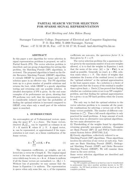
PARTIAL SEARCH VECTOR SELECTIONFOR SPARSE SIGNAL REPRESENTATIONKarl Skretting and John Håkon HusøyStavanger University College, Department of Electrical and Computer EngineeringP. O. Box 8002, N-4068 Stavanger, NorwayPhone: +47 51 83 20 16, Fax: +47 51 83 17 50, E-mail: karl.skretting@tn.his.noABSTRACTIn this paper a new algorithm for vector selection insignal representation problems is proposed, we call itPartial Search (PS). The vector selection problem isdescribed, and one group of algorithms for solving thisproblem, the Matching Pursuit (MP) algorithms, isreviewed. The proposed algorithm is based on the OrderRecursive Matching Pursuit (ORMP) algorithm,it extends ORMP by searching a larger part of thesolution space in an effective way. The PS algorithmtests up to a given number of possible solutions andreturns the best, while ORMP is a greedy algorithmtesting and returning only one possible solution. Adetailed description of PS is given. In the end someexamples of its performance are given, showing thatPS performs very well, that the representation erroris considerable reduced and that the probability offinding the optimal solution is increased compared toORMP, even when only a small part of the solutionspace is searched.1. INTRODUCTIONAn overcomplete set of N-dimensional vectors, spanningthe space R N , is a frame. The frame vectors,denoted {f k } K k=1, can be regarded as columns in anN × K matrix F, where K ≥ N. A signal vector,x, can be represented, or approximated if the representationis not exact, as a linear combination of theframe vectors,˜x =K∑w(k)f k = F w. (1)k=1The expansion coefficients, or weights, are collectedinto a vector w of length K. The original signalvector is the sum of the signal approximation and anerror which may be zero, x = ˜x+r. A frame is uniformif all the frame vectors are normalized, i.e. ‖f k ‖ = 1.Without loss of generality we may assume that theframe in Equation 1 is uniform. The representationis sparse when only some few, say s, of the expansioncoefficients are non-zero, the sparseness factor S, isthen given by S = s/N.The vector selection problem (for a sparseness factorgiven by the maximum number of non-zero weightsallowed, s) is to find the weights in Equation 1 suchthat the norm of the error, ‖r‖ = ‖x − Fw‖, is assmall as possible. Generally no exact, x = Fw, solutionexists when s < N. The choice of weights thatminimizes the 2-norm of the residual (error) is calledthe “optimal solution” or the optimal approximationin the least squares sense. An ɛ-solution is a choice ofweights such that the 2-norm of the residual is smallerthan a given limit, ɛ. Davis [1] has proved that findingwhether an ɛ-solution exists or not is an NP-complete 1problem, and that finding the optimal approximationfor a given s is an NP-hard problem when the 2-normis used.The only way to find the optimal solution to thevector selection problem is to examine all the possiblecombinations for selecting s vectors out of the Kframe vectors available. The number of different combinationsis ( )Ks . Thus a full search algorithm is onlypractical for small problems. A large amount of workhas been done on alternative non-optimal algorithms,the two main alternatives are:1) Thresholding of the weights found by algorithmsreturning generally non-sparse solutions. Examplesare Basis Pursuit (BP) [2] and FOCal Under-determinedSystem Solver (FOCUSS) [3,4].2) Greedy algorithms, collectively referred to asMatching Pursuit (MP) algorithms. These algorithmsinvolves the selection of one vector at each step. Variantsare Basic Matching Pursuit (BMP), OrthogonalMatching Pursuit (OMP) and Order RecursiveMatching Pursuit (ORMP). We will examine themcloser in the next section.Some vector selection algorithms are described andcompared in [5-7].1 An NP-complete problem is as hard as (can be transformedin polynomial time into) another problem known to be NPcomplete.An NP-hard problem is at least as hard as an NPcompleteproblem.

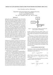
Basic Matching Pursuit (BMP) algorithm:1 w = BMP(F, x, s)2 w := 0, r := x3 while not Finished4 c := F T · r5 find k : |c(k)| = max j |c(j)|6 w(k) := w(k) + c(k)7 r := r − c(k) · f k8a Finished := (‖r‖ < some Limit)8b Finished := (s non-zero entries in w)9 end10 returnFigure 1: The Basic Matching Pursuit algorithm.In this paper we present the partial search methodfor vector selection. It may be seen as a reduction ofthe full search method, instead of searching all thepossible combinations it only searches the combinationscontaining the most promising frame vectors.Alternatively it may be seen as an extension of theORMP method: Instead of only selecting the mostpromising frame vector in each step, it may try severalframe vectors in each step. The proposed algorithmuse QR factorization the same way as the fast variantsof OMP and ORMP. The partial search method wasfirst presented as a recursive function without the fastQR factorization in [8]. In Section 2 we present theMP algorithms and the proposed algorithm for partialsearch is described in Section 3. In Section 4 some implementationdetails for the fast variants based on QRfactorization are presented. And finally, in Section 5,some numerical examples illustrate the performanceof PS compared to BMP, OMP and ORMP.2. MATCHING PURSUIT ALGORITHMSThe simplest of the Matching Pursuit algorithms isBasic Matching Pursuit (BMP), presented and analyzedin [1] and [9]. An overview of the algorithm isin Figure 1. This variant of the BMP algorithm aswell as the other algorithms presented here, requiresthat the frame, F, is uniform. The BMP algorithmhas the following four main steps: Initialize, Loop,Select and Update.In the initialize step the weights, w, are set tozero, and the residual, i.e. the representation errorusing the current weights, r = x − Fw, is set to thegiven signal vector, line 2 in Figure 1. The main loop,line 3-9, is done until some stop criterion is met. Itmay be that the representation error is small enough,line 8a, or that the desired number of non-zero entriesin w is reached, line 8b, or that the loop has beenexecuted many times, this third test is not includedin Figure 1.A (new) frame vector is selected to be used in thelinear combination which makes up the approximation.As this is a greedy algorithm we select the vectorthat looks best at the current stage. Within theloop the inner products of the current residual and theframe vectors are calculated, line 4, and the one withthe largest absolute value is identified, line 5. Framevector k is selected. It may happen that this is a vectorselected earlier, and thus the number of non-zeroentries in w is not increased but one of the alreadyselected entries is updated and the error is reduced.In fact, we may use this to reduce the error withoutselecting new frame vectors (as long as the error isnot orthogonal to the space spanned by the selectedframe vectors) by only considering the frame vectorsalready selected in line 5.The weight for the selected frame vector is updated,line 6, and the residual is updated, line 7. Weshould note that the calculation in line 7 makes theresidual orthogonal to the frame vector just selected,but it also add components in the same directions aspreviously selected frame vectors since these are notorthogonal to the frame vector just selected.The BMP algorithm is quite simple, but it is notvery effective. The loop may be executed many times,often more than s times, and the calculation of theinner products, line 4, is demanding, approximatelyNK multiplications and additions are done.Orthogonal Matching Pursuit (OMP) [1,10] isa refinement of BMP. The only difference is in the updatestep, line 6 and 7 in Figure 1. The approximationafter a new frame vector has been selected is made byprojecting the signal vector onto the space spannedby the selected frame vectors. When i frame vectorsare selected the index set of the selected frame vectorsis denoted I = {k 1 , k 2 , . . . , k i } and they are collectedinto a matrix A = [f k1 , f k2 , . . . , f ki ] of size N × i. Theapproximation is ˜x = A(A T A) −1 A T x = Ab and theerror is as before r = x − ˜x. Here, b = (A T A) −1 A T xis the values of the non-zero entries in w given by theindex set I. With this change the residual will alwaysbe orthogonal to the selected frame vectors, and theselect step will always find a new vector. This ensuresthat the loop is at most executed s times, but,in a straight forward implementation, the orthogonalizationof the residual add extra calculations to theloop.Order Recursive Matching Pursuit (ORMP)[12-15] is another MP variant. Like OMP this onealways keeps the residual orthogonal to all the selectedframe vectors. The only difference between ORMPand OMP is that ORMP adjust the inner productsbefore the largest is found, line 5 in Figure 1 will be“find k : |c(k)/u(k)| = max j |c(j)/u(j)|” instead of“find k : |c(k)| = max j |c(j)|”. Let us explain this in

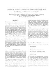
• i = 0• • •k (1)1 k (4)1 k (6)1• • • • • •k (1)2 k (2)2 k (3)2 k (4)2 k (5)2 k (6)2• • • • • •k (1)3 k (2)3 k (3)3 k (4)3 k (5)3 k (6)3I (1) I (2) I (3) I (4) I (5) I (6)i = 1i = 2i = 3Figure 2: Search tree for the example in Section 3.more detail:We denote the subspace of R N spanned by the columnvectors in A, i.e. the selected frame vectors, asA, and its orthogonal complement as A ⊥ . A framevector, f j , can be divided into two orthogonal components,the part in A of length a(j), and the partin A ⊥ of length u(j), and a(j) 2 + u(j) 2 = ‖f j ‖ 2 = 1,where the latter equality follows since the frame isuniform. Lengthening each remaining or not yet selectedframe vector f j by a factor 1/u(j), makes thelengths of the component in A ⊥ equal to 1. Thispart is the only one we need to consider since theresidual, r, is in A ⊥ . Thus, finding maximum of|c(j)|/u(j) = (fj T r)/u(j) = (f j T /u(j))r, instead ofonly |c(j)|, when selecting the next frame vector islike selecting a vector from a uniform frame in A ⊥ ,i.e. the frame vectors are orthogonalized to A and normalized.ORMP will generally select different framevectors than OMP, and often the total residual willbe smaller. A ”straight forward” implementation ofORMP will be even more demanding than OMP.3. THE PARTIAL SEARCH ALGORITHMThe idea of the Partial Search (PS) algorithm is tosearch many combinations, i.e. many sets of framevectors, to find the best solution. In PS we let thenumber of combinations, NoC, to search be given asan input argument. A particular combination, numberedm, has index set I (m) = {k (m)1 , k (m)2 , . . . , k s (m) }and the matrix of the selected frame vectors is denotedA (m) . Each combination gives an error, r (m) =x − ˜x (m) = x − A (m) (A (m)T A (m) ) −1 A (m)T x. Theindex set that gives the smallest error also gives thesolution, i.e. the sparse weights as in OMP.The different combinations can be ordered in asearch tree as in Figure 2, here NoC = 6. Each node,except the root, in the tree represent the selection ofone frame vector. The index set given by each leaf isgiven by the path from the root to the leaf. An indexset may have the same start for the index sequence asanother index set, i.e. k (3)1 = k (2)1 = k (1)1 and k (5)1 =. In the PS algorithm the tree is searched in ak (4)1depth-first way. The current state is saved each time,on the way down, a node with more than one childis reached, and on the way up the state is retrievedbefore visiting the next child. At each leaf the norm ofthe error is calculated and compared to the smallesterror found until now.One important part of the PS algorithm is to decidewhich frame vectors to select, the indexes k (m)i toinclude in the search tree. A function, named “DistributeM”,does this task each time a new node isvisited, starting at the root where i = 0 and at allthe levels down to i = s − 1. This function distributethe number of combinations available M, at the root(i = 0) this is M = NoC, by returning a sequenceof non-negative integers, M k for k = 1, 2, . . . , K, suchthat∑M k > 0 if frame vector k is to be included andKk=1 M k = M. M k is used as the M value at thenext level. This is done according to the rules decidedwhen building the function and it always uses the innerproducts c (actually the adjusted inner productsd where d(j) = |c(j)|/u(j) since the ORMP variant isthe preferred one), and M. The function may also dependon the number of vectors already selected i, themaximum number of vectors to select s, or the framesize N and K. The best (criterium as in ORMP)frame vector should be the first one, and thus makesure that the ORMP index set is I (1) , also the selectedindexes should be the best ones in d. In the examplein Figure 2 NoC = 6 combinations are availableat the root, these are distributed so that M (1) k= 3,1M (4) k= 2 and M (6)1k= 1 and M k = 0 for the rest1of the k’s. At level i = 1 and for node k (1)1 theM = 3 combinations to search are distributed suchthat M (1) k= 1, M (2)2k= 1 and M (3)2k= 1.2We can note that all the leafs in the tree are atlevel i = s and that none of the leafs has any siblings.At level i = s − 1 it makes no sense to try more thanthe best frame vector since this is the one that willgive the smallest error.An effective implementation of the PS algorithmshould exploit the tree structure to avoid doing thesame calculations several times. It is also importantthat as few calculations as possible is done to find thenorm of the error at each leaf, it is not necessary toform the matrices A (m) nor to do matrix inversion.The same technique as used in QR factorization inOMP and ORMP can be applied in the PS algorithm.The details are in the next section.

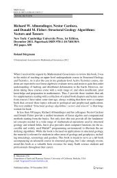
OMP/ORMP with QR factorization:1 w = OMPqr/ORMPqr(F, x, s)2 R := 03 i := 0, I := {}, J := {1, 2, . . . , K}4 e := 1, u := 15 c := F T x, d := |c|6 nx := x T x, nxLim := nx · 10 −107 while 18 find k : d(k) = max j d(j)9 i := i + 1, I := I ∪ {k}, J := J \ {k}10 R(i, k) := u(k)11 nx := nx − c(k) 212 if (i ≥ s) or (nx < nxLim) exit loop13 for j ∈ J14 R(i, j) := fk T f j15 for n := 1 to (i − 1)16 R(i, j) := R(i, j) − R(n, k)R(n, j)17 end18 R(i, j) := R(i, j)/u(k)19 c(j) := c(j)u(j) − c(k)R(i, j)20 if OMP d(j) := |c(j)|21 e(j) := e(j) − R(i, j) 222 u(j) := √ |e(j)|23 c(j) := c(j)/u(j)24 if ORMP d(j) := |c(j)|25 end26 d(k) := 027 end28 w := 029 w(I) := R(1 : i, I) −1 c(I)30 returnFigure 3: The OMP/ORMP algorithm using QR factorization.Partial Search with QR factorization:1 w = PSqr(F, x, s, NoC)2 Initialize R, M, e, u, c, d, nx, nxLim,nxBest, GoingDown, i, I and J3 while 14 if GoingDown5 increment i6 find k : d(k) = max j d(j)7 call “DistributeM” function8 if “two or more children” store state9 end10 GoingDown = true11 I := I ∪ {k}, J := J \ {k}12 R(i, k) := u(k)13 nx := nx − c(k) 214 if (nx < nxLim) find w by backsubstitutionand exit loop15 if (i < s)16 Update R(i, J), c, d, e and u17 else18 if (nx < nxBest) update nxBest andfind w by back-substitution19 decrement i, set I, Juntil (“sibling” found) or (i = 0)20 if (i = 0) exit loop21 set k to index of “sibling”22 retrieve state23 GoingDown = false24 end25 end26 returnFigure 4: The Partial Search algorithm using QR factorization.More explanation in text.4. IMPLEMENTATION DETAILSFast algorithms based on QR factorization havebeen presented for both OMP and ORMP, [1,13,15].One such algorithm is given in Figure 3. QR factorizationis done on the matrix of the selected framevectors, denoted A above. Actually the Q matrix isnot explicitly formed, only the R matrix is stored.QR factorization is done as in the stable ModifiedGram-Schmidt algorithm [15], after the selection of anew frame vector all the remaining frame vectors areorthogonalized to the one just selected.We will now look closer into the algorithm shownin Figure 3. The matrix R is of size s×K, where R(1 :i, I) is the R matrix in QR factorization of matrix A.I is the index set for the selected vectors and J is theindex set of the remaining frame vectors. The vectorse, u, c and d in line 4 and 5 are all of length K, e(k) isthe length squared of f k projected into A ⊥ and u(k)is the length. c contains the inner products of theframe vectors and the residual, and d theirs absolutevalues (OMP) or the absolute values diveded by thelengths u(k) (ORMP). nx will be updated in line 11to be nx = ‖r‖ 2 after the selection of each new framevector.The main loop, line 7-27, selects one frame vectoreach time it is executed, line 8 and 9. If allowed numberof vectors are selected, or the norm of the residualis small, the loop is ended. To prepare for selectionof more frame vector more work is needed, line 13-26.First (entries for unselected frame vectors in) row i ofR is updated, line 14-18, then vectors c, d, e and uare updated, line 19-24. Finally, d(k) is set to zero toensure that new vectors are selected. When then desired(or needed) number of frame vectors are selecteda linear equation system must be solved to find theweights. Since the matrix R(1 : i, I) is triangular thiscan be solved quite simply by backward substitution,line 29.The kernel of the PS algorithm is ORMPqr, it iswrapped in a walk through the search tree. The PS

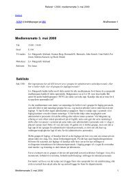
1621Frame F 1SNR value141210811.34s=69.17s=514.5513.5911.1910.748.17 8.32SNR value2019181716Frame F 2s=9s=718.4917.2919.1617.9916.3319.9318.5716.766s=47.17s=3 5.345.86 5.8815s=515.634BMP OMP ORMP PS,20 100 500 500014BMP OMP ORMP PS,20 100 500 5000Figure 5: The approximation errors for the randomGaussian data using the “random” frame F 1 .Figure 6: The approximation errors for the AR(1)signal vectors using the “designed” frame F 2 .algorithm is summarized in Figure 4. Initializationin line 2 is like line 2-6 in Figure 3, but some fewextra variables are included. M is a matrix or a tableused to store the different M values found by the“DistributeM” function. The state stored in line 8and retrieved in line 22 is the variables c, e, u andnx. Note that the state is assumed to be stored ina table, where i is the position, that allows a statestored once to be retrieved several times. Line 16 updatesR(i, J), c, d, e and u like line 13-26 in Figure 3.When the walk through the search tree has reached aleaf lines 18-23 are executed, we go up in the searchtree (decrement i) until a sibling to the right of thecurrent node is found. The search is finished whenthe root is reached.5. SIMULATION EXAMPLESIn this section we will give some examples of the performanceof the Partial Search (PS) algorithm. Thevector selection algorithms that will be used are BMP,OMP, ORMP, and Partial Search with the allowednumber of combinations to search, NoC, set as 20,100, 500 and 5000. The methods will be along thex-axis in Figures 5 and 6. For a given sparseness factorthe results of BMP, OMP and ORMP are looselyconnected by a dotted line and the results of ORMPand PS with different values for NoC are connectedby a solid line since here intermediate values can beassumed using different values for NoC. Note thatORMP can be regarded as PS with NoC = 1.Having a set of L test vectors, x l for l = 1 toL, we find sparse approximations to each of the testvectors using the different vector selection methods.The ideal situation now would be if we could comparethese results to the optimal solution, but this is onlypossible for very small problems. Thus we can notfind for how many of these L test vectors the optimalsolution were found, or how close the resulting error isto the error of the optimal solution. The approximationerror for each test vector can be used to comparethe different methods to each other. It can be quantifiedby the Signal to Noise Ratio (SNR) defined (eg.estimated) as∑ Ll=1SNR = −10 log ‖r l‖ 210 ∑ Ll=1 ‖x l‖ = −10 log E r2 10 (2)E xwhere r l = x l − ˜x l and the 2-norm is used. The denominatorin this fraction is constant for a given setof test vectors. Thus, an increase in the SNR value by1 is a reduction of the energy in the error, E r , by 20%.The SNR will be along the y-axis in Figures 5 and 6.As more combinations are searched, NoC increases,the optimal solution is more likely to be found, andthe total approximation error will be smaller (higherSNR). When a (considerable) increase in NoC doesnot give a higher SNR we may expect that the optimalsolution is found for most of the test vectors.In the first example a set of L = 5000 randomGaussian vectors is generated. The test vectors areof length N = 16, each entry is independent andGaussian distributed (zero mean and variance σ = 1).Each of these vectors is approximated by a sparse representation,s = 3, . . . , 6 frame vectors were used forthese approximations. The frame vectors in F 1 , size16 × 48, are selected similar to the test vectors, i.e.they are random Gaussian vectors which are normalized,‖f k ‖ = 1. The results are presented in Figure 5.It is perhaps more interesting to look at the vectorselection capabilities for not completely randomsignals. This is done in the second example. A long

AR(1) signal 2 , with ρ = 0.95 is divided into L = 5000non-overlapping blocks, each with length N = 32,these make up the other set of test vectors, whichin Figure 6 is approximated by a sparse representationusing s = 5, 7 or 9 frame vectors. The frameF 2 , of size 32 × 80, is a frame specially designed forAR(1) signals, the frame design method is describedin [8]. The sparse representation results are presentedin Figure 6.The conclusions we can draw from these examplesare: 1) Comparing the MP algorithms we see thatOMP and ORMP both give better approximationsthan BMP, and that ORMP is the better one. 2)The PS algorithm is considerable better than the MPalgorithms, already for NoC = 20 the probability offinding a better (the optimal) solution is considerablehigher. 3) For values of s ≤ 5, or not a large numberof different possible combinations ( Ks), it seems thatPS is likely to find the optimal solution with a smallor moderate value of NoC.One disadvantage of PS is that the execution timeis larger than for ORMP (and OMP). This can beseen in the following table for frame F 2 used on 5000test vectors with s = 9.frame F 2 , s = 9 Running Time for eachMethod Time combinationORMP, (NoC = 1) 3.23 s 3.23 sPS, NoC = 20 53.6 s 2.68 sPS, NoC = 100 4 min 9 s 2.49 sPS, NoC = 500 19 min 45 s 2.37 sPS, NoC = 5000 3 h 13 min 2.32 sThe execution time increases almost linearly with thenumber of combinations searched. The time for searchingone combination decreases as more combinationsare searched, this is natural since a new combinationusually has some of the first vectors in common withthe previously searched combination, and this is exploitedit the algorithm.6. CONCLUSIONThe partial search algorithm presented in this paperfinds a solution to the vector selection problem at leastas good as the ORMP algorithm. The optimal solutionis often found by searching relatively few combinations,often 20 to 100 combinations seems enough.The search among the different combinations is donein a fast and effective way. The improvement in representationwhen going from ORMP to partial searchis the same size as the improvement when going fromBMP to ORMP, or better if we allow to search manycombinations.7. REFERENCES[1] G. Davis, Adaptive Nonlinear Approximations, Ph.D.thesis, New York University, Sept. 1994.[2] S. S. Chen, D. L. Donoho, and M. A. Saunders, “Atomicdecomposition by basis pursuit,” SIAM Journal of ScientificComputing, vol. 20, no. 1, pp. 33–61, 1998.[3] I. F. Gorodnitsky and B. D. Rao, “Sparse signal reconstructionfrom limited data using FOCUSS: A re-weightedminimum norm algorithm,” IEEE Trans. Signal Processing,vol. 45, no. 3, pp. 600–616, Mar. 1997.[4] K. Engan, Frame Based Signal Representation and Compression,Ph.D. thesis, Norges teknisk-naturvitenskapeligeuniversitet (NTNU)/Høgskolen i Stavanger, Sept. 2000,Available at http://www.ux.his.no/˜kjersti/.[5] B. D. Rao, “Signal processing with the sparseness constraint,”in Proc. ICASSP ’98, Seattle, USA, May 1998,pp. 1861–1864.[6] B. D. Rao and K. Kreutz-Delgado, “Sparse solutionsto linear inverse problems with multiple measrement vectors,”in Proc. DSP Workshop, Bryce Canyon, Utah, USA,Aug. 1998.[7] S. F. Cotter, J. Adler, B. D. Rao, and K. Kreutz-Delgado,“Forward sequential algorithms for best basis selection,”IEE Proc. Vis. Image Signal Process, vol. 146, no. 5, pp.235–244, Oct. 1999.[8] K. Skretting, Sparse Signal Representation using OverlappingFrames, Ph.D. thesis, NTNU Trondheimand Høgskolen i Stavanger, Oct. 2002, Available athttp://www.ux.his.no/˜karlsk/.[9] S. G. Mallat and Z. Zhang, “Matching pursuit with timefrequencydictionaries,” IEEE Trans. Signal Processing,vol. 41, no. 12, pp. 3397–3415, Dec. 1993.[10] Y. C. Pati, R. Rezaiifar, and P. S. Krishnaprasad, “Orthogonalmatching pursuit: Recursive function approximationwith applications to wavelet decomposition,” Nov.1993, Proc. of Asilomar Conference on Signals Systemsand Computers.[11] S. Singhal and B. S. Atal, “Amplitude optimizationand pitch prediction in multipulse coders,” IEEE Trans.Acoust., Speech, Signal Processing, vol. 37, no. 3, pp. 317–327, Mar. 1989.[12] S. Chen and J. Wigger, “Fast orthogonal least squares algorithmfor efficient subset model selection,” IEEE Trans.Signal Processing, vol. 43, no. 7, pp. 1713–1715, July 1995.[13] B. K. Natarajan, “Sparse approximate solutions to linearsystems,” SIAM journal on computing, vol. 24, pp. 227–234, Apr. 1995.[14] M. Gharavi-Alkhansari and T. S. Huang, “A fast orthogonalmatching pursuit algorithm,” in Proc. ICASSP ’98,Seattle, USA, May 1998, pp. 1389–1392.[15] L. N. Trefethen and D. Bau, Numerical Linear Algebra,Siam, Philadelphia, PA, USA, 1997.2 An AR(1) signal is the output of an autoregressive (AR)process of order 1.