Part 1 - AL-Tax
Part 1 - AL-Tax Part 1 - AL-Tax
appearance of future competitors attracted by extraordinary rents in the industry.Let us consider that assumption, and to model the pre-tax rate of return as a geometricBrownian motion with drift:dp αp dt σp dz (2.18)where dz is the increment of a Wiener process, α 1 is the drift parameter, andσ the variance parameter. Given that the project is expected to generate economicrents in the beginning, new similar projects will come and reduce the economicrent, a fact that is modeled with a negative trend.As an example of a geometric Brownian motion with negative drift, we presentin Figure 2.4 a sample path of equation (2.18) with a drift rate of 5% per year anda standard deviation of 25% per year. The graphic is built with monthly timeintervals.Now the expected NPV of the project is (see Dixit and Pindyck, 1994):and the expected NPVT:pE[ NPV* ] ⎡ E ptte( ρδπ )⎤0∫dt⎣⎢ 0⎦⎥ρδπ αChapter 2⎡ E[ NPVT ] E τ( ptt δ)e ( ρδπ )⎤∫dt A⎣⎢0⎦⎥τδπρδπ pA0 .ρδπα 0.140.120.100.080.060.040.020.0055 60 65 70 75 80 85 90 95 00Figure 2.4Geometric Brownian motion with negative drift25
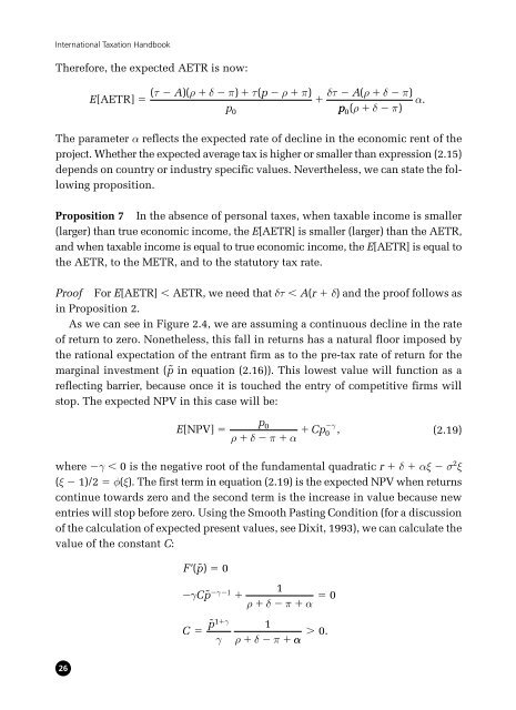
International Taxation HandbookTherefore, the expected AETR is now:( τ A)( ) ( p ) A( )E[ AETR] ρδπτ ρπδτ ρδπ α.pp 0 ( ρδπ )The parameter α reflects the expected rate of decline in the economic rent of theproject. Whether the expected average tax is higher or smaller than expression (2.15)depends on country or industry specific values. Nevertheless, we can state the followingproposition.Proposition 7 In the absence of personal taxes, when taxable income is smaller(larger) than true economic income, the E[AETR] is smaller (larger) than the AETR,and when taxable income is equal to true economic income, the E[AETR] is equal tothe AETR, to the METR, and to the statutory tax rate.Proof For E[AETR] AETR, we need that δτ A(r δ) and the proof follows asin Proposition 2.As we can see in Figure 2.4, we are assuming a continuous decline in the rateof return to zero. Nonetheless, this fall in returns has a natural floor imposed bythe rational expectation of the entrant firm as to the pre-tax rate of return for themarginal investment (p˜ in equation (2.16)). This lowest value will function as areflecting barrier, because once it is touched the entry of competitive firms willstop. The expected NPV in this case will be:p0E[ NPV ] Cp0 γ,ρδ π α(2.19)where γ 0 is the negative root of the fundamental quadratic r δαξ σ 2 ξ(ξ 1)/2 φ(ξ). The first term in equation (2.19) is the expected NPV when returnscontinue towards zero and the second term is the increase in value because newentries will stop before zero. Using the Smooth Pasting Condition (for a discussionof the calculation of expected present values, see Dixit, 1993), we can calculate thevalue of the constant C:F( pɶ) 00 Cp 1γ ɶ γ 1 0ρδπα pɶ1γ1C γρδπ α 0.26
- Page 2 and 3: International TaxationHandbook
- Page 4 and 5: International TaxationHandbookPolic
- Page 6 and 7: ContentsAbout the editorsAbout the
- Page 9 and 10: Contents7.3 Between routine risk an
- Page 11 and 12: Contents10.3 The theoretical litera
- Page 13 and 14: Contents15.3 Competitive equilibriu
- Page 16 and 17: About the contributorsDr Paul U. Al
- Page 18 and 19: About the contributorsLouvain-la-Ne
- Page 20 and 21: About the contributorsCésar August
- Page 22: Part 1International TaxationTheory
- Page 25 and 26: This page intentionally left blank
- Page 27 and 28: International Taxation Handbookinto
- Page 29 and 30: International Taxation Handbookempi
- Page 31 and 32: International Taxation HandbookThis
- Page 33 and 34: This page intentionally left blank
- Page 35 and 36: International Taxation HandbookMarg
- Page 37 and 38: International Taxation HandbookrS
- Page 39 and 40: International Taxation Handbooka gr
- Page 41 and 42: International Taxation HandbookIt f
- Page 43 and 44: International Taxation Handbookthat
- Page 45: International Taxation HandbookProp
- Page 49 and 50: International Taxation Handbookther
- Page 51 and 52: International Taxation Handbook2.3.
- Page 53 and 54: International Taxation Handbookprod
- Page 55 and 56: International Taxation Handbookinpu
- Page 57 and 58: International Taxation HandbookThe
- Page 59 and 60: International Taxation HandbookRefe
- Page 61 and 62: International Taxation Handbook●
- Page 63 and 64: This page intentionally left blank
- Page 65 and 66: This page intentionally left blank
- Page 67 and 68: International Taxation Handbookconf
- Page 69 and 70: International Taxation Handbookelab
- Page 71 and 72: International Taxation Handbookthei
- Page 73 and 74: International Taxation Handbookτ*
- Page 75 and 76: International Taxation Handbookwher
- Page 77 and 78: International Taxation Handbookcoun
- Page 79 and 80: International Taxation Handbookown
- Page 81 and 82: International Taxation Handbookand
- Page 83 and 84: International Taxation Handbookand
- Page 85 and 86: 64Table 3.2Capital tax rates and in
- Page 87 and 88: International Taxation HandbookHays
- Page 89 and 90: International Taxation Handbookpape
- Page 91 and 92: International Taxation Handbookthat
- Page 93 and 94: International Taxation HandbookSwan
- Page 95 and 96: This page intentionally left blank
International <strong>Tax</strong>ation HandbookTherefore, the expected AETR is now:( τ A)( ) ( p ) A( )E[ AETR] ρδπτ ρπδτ ρδπ α.pp 0 ( ρδπ )The parameter α reflects the expected rate of decline in the economic rent of theproject. Whether the expected average tax is higher or smaller than expression (2.15)depends on country or industry specific values. Nevertheless, we can state the followingproposition.Proposition 7 In the absence of personal taxes, when taxable income is smaller(larger) than true economic income, the E[AETR] is smaller (larger) than the AETR,and when taxable income is equal to true economic income, the E[AETR] is equal tothe AETR, to the METR, and to the statutory tax rate.Proof For E[AETR] AETR, we need that δτ A(r δ) and the proof follows asin Proposition 2.As we can see in Figure 2.4, we are assuming a continuous decline in the rateof return to zero. Nonetheless, this fall in returns has a natural floor imposed bythe rational expectation of the entrant firm as to the pre-tax rate of return for themarginal investment (p˜ in equation (2.16)). This lowest value will function as areflecting barrier, because once it is touched the entry of competitive firms willstop. The expected NPV in this case will be:p0E[ NPV ] Cp0 γ,ρδ π α(2.19)where γ 0 is the negative root of the fundamental quadratic r δαξ σ 2 ξ(ξ 1)/2 φ(ξ). The first term in equation (2.19) is the expected NPV when returnscontinue towards zero and the second term is the increase in value because newentries will stop before zero. Using the Smooth Pasting Condition (for a discussionof the calculation of expected present values, see Dixit, 1993), we can calculate thevalue of the constant C:F( pɶ) 00 Cp 1γ ɶ γ 1 0ρδπα pɶ1γ1C γρδπ α 0.26


