Chapter 3. Probability

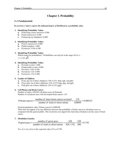
Chapter 3: Probability 633–2 FundamentalsChapter 3. ProbabilityIn exercises 1 and 2, express the indicated degree of likelihood as a probability value.1. Identifying Probability Valuesa. P(choosing correct answer)= 0.500b. P(rain tomorrow)= 0.200c. P(marrying my daughter)= 0.0002. Identifying Probability Valuesa. P(snow tomorrow)= 0.900b. P(dark tonight)= 1.000c. P(correct)= 1/10= 0.1003. Identifying Probability ValuesWhich cannot be probabilities? Probabilities can only be in the range of 0 to 1.-1, 2, 5/3, 24. Identifying Probability Valuesa. P(certain event)= 1.000b. P(impossible event)= 0.000c. P(event)= 1/10= 0.100d. P(correct)= 1/2= 0.500e. P(correct)= 1/5= 0.2005. Gender of Childrena. P(one girl out of three children)= 3/8= 0.375 (bbg, bgb, and gbb)b. P(two girls out of three children)= 3/8= 0.375 (bgg, gbg, and ggb)c. P(all girls out of three children)= 1/8= 0.125 (ggg)6. Cell Phones and Brain CancerNumber of trials= 420,095 cell phone users in DenmarkNumber of cell phone users who developed brain cancer= 135number of times brain cancer occurred 135P ( brain cancer) == = 0.000321number of trials or observations 420095General population value, P(brain cancer)= 0.000340There does not appear to be any difference between the probability of brain cancer in cell phone users ascompared with the general public. This result does not support the claim that cell phones are the cause of braincancer.7. Mendelian Geneticsnumber of green peas 428 428P ( green pea) == = = 0.738number of trials or observations 428 + 152 580Yes, it is very close to the expected value of ¾ or 0.750.

64 Chapter 3: Probability8. Being Struck by LighteningNumber struck per year= 389, People in US during that year= 28,142,906P(struck by lightening this year) =389281,421,906= 0.00000138number of those struck by lighteningnumber in population=Using Probability to Identify Unusual Events. In exercises 9-12 consider an event to be “unusual” if itsprobability is less than or equal to 0.05. (This is equivalent to the same criterion commonly used in inferentialstatistics, but the value of 0.05 is not absolutely rigid, and other values such as 0.01 are sometimes used instead.)9. Probability of a Wrong Eventnumber of wrong events 5a. P ( wrong) == = 0. 0588number of trials or observations 85b. Since P= 0.0588 is greater than 0.05, it is not “unusual” for this test conclusion to bewrong for women who are pregnant.10. Probability of Wrong Resultnumber of wrong results 3a. P ( wrong result) == = 0. 214number of trials or observations 14b. Since P= 0.214 is greater than 0.05, it is not “unusual” for this test conclusion to bewrong for women who are not pregnant.11. Cholesterol-Reducing Drugnumber of flu symptom events 19 19a. P ( flu symptoms) == = = 0. 0220number of trials or observations 19 + 844 863b. Since P= 0.0220 is less than 0.05, it is considered “unusual” for patients taking this drug to experience flusymptoms.12. Guessing Birthdaysnumber of ways correct birthday can occur 1a. P (guessing birthday) == = 0. 00274number of different days 365b. Since P= 0.00274 is less than 0.05, it is considered “unusual” for Mike to guess Kelly’s birthday correctly.c. This would be such a good guess or unusual outcome that it would be reasonable to believe that Mike mayhave already known Kelly’s birthday, but it is possible that this was a good guess.d. Guessing another person’s age and being 15 years over the estimate is not flattering to anyone. In this case,Mike is not likely to get another date, but it’s not impossible.13. Probability of a Birthdaynumber of ways correct birthday can occur 1a. P ( correct) == = 0. 00274number of different days 365

Chapter 3: Probability 65number of ways correct October birthday can occur 31b. P ( correct) == = 0. 0849number of different days365number of ways birthday ends in y 7c. P ( correct) == = 1. 000number of different days in week 714. Probability of a Car Crashnumber of times 20 - 24 year old is in car crash 136P ( in car crash) == = 0.340number of drivers observed in sample 400While we don’t have the probabilities for other age groups, it would be reasonable to conclude that thisprobability is high enough to be of concern to 20-24 year olds.15. Probability of an Adverse Drug Reactionnumber of times headache occurred 117 117P ( headache) == = = 0.159number of times patients observed 117 + 617 734Yes, this probability of about 16 times out of 100 patients would be of concern to many Viagra patients.16. Gender of Children: Constructing Sample Spacea. Possible Outcomes: girl-girl, girl-boy, boy-girl, boy-boynumber of ways both girls can occur 1b. P ( both girls) == = 0. 250number of different possible outcomes 4number of ways one of each sex can occur 2c. P ( one of each sex) == = 0. 500number of different possibleoutcomes 417. Genetics: Constructing Sample Space, both with blue-brown, brown dominanta. Possible Outcomes, blue-blue= blue, blue-brown= brown, brown-blue= brown, brown-brown= brownnumber of ways blue eyes can occur 1b. P ( blue) == = 0. 250number of different possible outcomes 4number of ways brown eyes can occur 3c. P ( brown) == = 0. 750number of different possible outcomes 418. Genetics: Constructing Sample Space, one with brown-brown and one with brown-blue, brown dominanta. Possible Outcomes, brown-brown= brown, brown-blue= brown, brown-brown= brown, brown-blue=brownnumber of ways blue eyes can occur 0b. P ( blue ) == = 0. 000number of different possible outcomes 4number of ways brown eyes can occur 4c. P ( brown) == = 1. 000number of different possible outcomes 4

66 Chapter 3: Probability19. Genetics: Sample Space, one with brown-brown and one with blue-blue, brown dominanta. Possible Outcomes, brown-blue= brown, brown-blue= brown, brown-blue= brown, brown-blue= brownnumber of ways blue eyes can occur 0b. P ( blue) == = 0. 000number of different possible outcomes 4number of ways brown eyes can occur 4c. P ( brown ) == = 1. 000number of different possible outcomes 420. Improving Effectiveness of a TreatmentIf the probability is 0.04 that the treatment group would show improvement when the drug is not effective, wewould conclude that it is likely the drug is effective. There would be a probability of 0.04 of being wrong inconcluding the drug was effective.3-3 Addition RuleDetermining Whether Events Are Disjoint. For each part of exercises 1 and 2, are the two events disjoint for asingle trial? (Hint: Consider “disjoint” to be equivalent to “separate” or “not overlapping.”)This is also referred as being “mutually exclusive” where both events cannot occur at the same time.1. a. Not disjoint, since a cardiac surgeon could also be a female physician.b. Not disjoint, since a female college student could also drive a motorcycle.c. Disjoint, since if a study subject received Lipitor, he/she could not also be in a control group that receivedno medication.2. a. Disjoint, since a fruit fly cannot have both red and sepia colored eyes.b. Disjoint, since a volunteer survey subject can both oppose all cloning and approve cloning sheep.c. Not disjoint, since a nurse could also be male.3. Finding ComplementsThe complement of the probability of an event is the probability that that even will not occur.The sum of a probability and its complement is equal to 1.a. If P(A)= 0.05, then P( A )= 1 – 0.05= 0.95b. If probability of having red/green blindness is 0.25% or 0.0025, then the probability of not having red/greenblindness is 1 – 0.0025= 0.9975.4. Finding Complementsa. If P(A)= 0.0175, then P( A )= 1.0000 – 0.0175= 0.9825b. If 61% believe in life elsewhere, then P(believe in life elsewhere)= 0.61 and P(do not believe)= 1.00 –0.610= 0.3905. Peas on Earth, based on Table 3-2P(green pod or white flower)= P(green pod) + P(white flower) – P(both green pod and white flower) = 8/14 +5/14 – 3/14= 10/14= 0.7146. Peas on Earth, based on Table 3-2P(yellow pod or purple flower)= P(yellow pod) + P(purple flower) – P(both yellow pod and purple flower) =6/14 + 9/14 – 4/14= 11/14= 0.7867. National Statistics DayP(birthday on Oct. 18)= 1/365, P(birthday not on Oct. 18)= 364/365= 0.997

Chapter 3: Probability 678. Birthday and ComplementP(birthday not in Oct.)= 1 – P(birthday in Oct.)= 1 – 31/365= 1 – 0.085= 0.915In Exercises 9-12, use the data in the following table, which summarizes results from the sinking of the Titanic.Men Women Boys Girls TotalSurvived 332 318 29 27 706Died 1360 104 35 18 1517Total 1692 422 64 45 22239. Titanic Passengers (n= 2223), this is a disjoint probabilityP(women or child)= P(women) + P(child)= 422/2223 + (64 + 45)/2223=0.1898 + 109/2223= 0.1898 + 0.0490= 0.23910. Titanic Passengers (n= 2223), this is not a disjoint probabilityP(man or survived)= P(man) + P(survived) – P(man and survived)=1692/2223 + 706/2223 – 332/2223= 0.7602 + 0.3176 – 0.1493= 0.92911. Titanic Passengers (n= 2223), this is not a disjoint probabilityP(child or survived)= P(child) + P(survived) – P(child and survived)=109/2223 + 706/2223 – (29 + 27)/2223= 0.0490 + 0.3176 – 56/2223=0.3660 – 0.0252= 0.34112. Titanic Passengers (n= 2223), this is not a disjoint probabilityP(woman or didn’t survive)= P(woman) + P(didn’t survive) – P(woman and didn’t survive)=422/2223 + 1517/2223 – 104/2223= 0.1898 + 0.6824 – 0.0468= 0.825In Exercises 13-20, use the data in the following table, which summarizes blood groups and Rh types for 100typical people. These values may vary in different regions according to the ethnicity of the population.Rh TypeO A B AB TotalPositive 39 35 8 4 86Negative 6 5 2 1 14Total 45 40 10 5 10013. Blood Groups and Types (n= 100), complementP( A )= 1 – P(A)= 1 – 40/100= 1 – 0.400= 0.60014. Blood Groups and Types (n= 100)P(Rh – )= 14/100= 0.14015. Blood Groups and Types (n= 100), not a disjoint probabilityP(A or Rh – )= P(A) + P(Rh – ) – P(A and Rh – )= 40/100 + 14/100 – 5/100=0.400 + 0.140 – 0.050= 0.49016. Blood Groups and Types (n= 100), a disjoint probabilityP(A or B)= P(A) + P(B)= 40/100 + 10/100= 0.400 + 0.100= 0.50017. Blood Groups and Types (n= 100), complementP(not Rh + )=1 – P(Rh – )= 1 – 14/100= 1 – 0.140= 0.86018. Blood Groups and Types (n= 100), not a disjoint probabilityP(B or Rh + )= P(B) + P(Rh + ) – P(B and Rh + )= 10/100 + 86/100 – 8/100=0.100 + 0.860 – 0.080= 0.880

68 Chapter 3: Probability19. Blood Groups and Types (n= 100), not a disjoint probabilityP(AB or Rh + )= P(AB) + P(Rh + ) = P(AB and Rh + )=5/100 +86/100 – 4/100=0.050 + 0.860 – 0.040= 0.87020. Blood Groups and Types (n= 100), not disjoint probabilitiesP(A or O or Rh + )=P(A) + P(O) + P(Rh + ) – P(A and Rh + ) – P(O and Rh + )=40/100 + 45/100 +86/100 – 35/100 – 39/100= 0.400 + 0.450 + 0.860 – 0.350 – 0.390=0.97021. Poll Resistance. A disjoint probabilityAge GroupResponded Didn’t Respond Total18-21 73 11 8422-29 255 20 275Total 328 31 359P(18-21 or didn’t respond)= P(18-21) + P(didn’t respond) – P(18-21 and didn’t respond)=84/359 + 31/359 – 11/359= 0.2340 + 0.0864 – 0.0306= 0.29022. Poll Resistance. A disjoint probabilityP(18-21 or responded)= P(18-21) + p(responded) – P(18-21 and responded)=84/359 + 328/359 – 73/359= 0.2340 + 0.9136 – 0.2033= 0.94423. Disjoint EventsNo. Take the events of: A is Pregnant, B is Male and C is Female. A (Pregnant) and B (Male) is disjoint,B(Male) and C(Female) is disjoint, but A(Pregnant) and C (Female) are not disjoint.24. Exclusive OrThe “exclusive or” implies that neither event can be included in the probability, thus the common probability,P(A and B), must be removed twice from the sum of the probabilities. The formula would be:P(A or B)= P(A) – P(A and B) + P(B) – P(A and B)= P(A) + P(B) – 2 P(A and B)3–4 Multiplication Rule: BasicsIdentifying Events as Independent or Dependent. In exercises 1 and 2, for each given pair of events, classify theevents as independent or dependent.1. a. Randomly selecting a grizzly bear and randomly selecting a male mammalIndependent, since the outcome of selecting a grizzly bear is not related to being a male mammal since thesecond selected Grizzly bear could be a female mammal.b. Randomly selecting a TV viewer who is watching The Living Planet and randomly selecting a second TVviewer who is watching The Living PlanetDependent, assuming that both TV viewers are in the same room with only 1 TV. Otherwise, they would beindependent if they were not in the same room with only 1 TV since the second person selected could bewatching something else.c. Wearing plaid shorts with black socks and sandals and asking someone on a date and getting a positiveresponseProbably dependent since wearing such attire might reduce the likelihood of getting a positive responsewhen asking for a date, but it could still happen.2. a. Finding that your calculator is not working and finding your refrigerator is not workingDependent, if both are operated using house current, but independent if the calculator was battery poweredand the refrigerator powered with house current.b. Finding out your kitchen light is not working and finding out refrigerator is not working

Chapter 3: Probability 69Dependent, since if both, as is likely to be the case, are using the same house current, these events would bedependent.c. Drinking until your driving ability is impaired and being involved in a car crashDependent, since impaired ability to drive increases the likelihood of having a car crash3. Coin and Die, independent eventsP(tail on coin and 3 on die)= P(tail) ∗ P(3)= 1/2 ∗ 1/6= 0.5000 ∗ 0.1667= 0.08334. Letter and Digit, independent eventsP(letter K and number 9)=P(K) ∗ P(9)= 1/26 ∗ 1/10= 0.0385 ∗ 0.1000= 0.004Pregnancy Test Results. In Exercises 5-8, use the data in Table 3-1.Table 3-1. Pregnancy Test ResultsPositive Test Result(Pregnancy is indicatedNegative Test Result(Pregnancy is not indicated)Subject is pregnant 80 5 85Subject is not pregnant 3 11 14Total 83 16 99Total5. Positive Test ResultP(first test +)= 83/99= 0.8384 (one positive test is removed from data set)P(second test+)= 82/98= 0.8367P(first and second tests are both +)= P(first test +) ∗ P(second test +)=0.8384 ∗ 0.8367= 0.7016. PregnantP(tests – or is not pregnant)= P(tests –) + P(not pregnant) – P(tests – and is not pregnant)=16/99 + 14/99 – 11/99= 0.1616 + 0.1414 – 0.1111= 0.1957. PregnantP( first subject is pregnant)= 85/99= 0.8586 (one pregnant subject is removed from data set)P(second subject is pregnant)= 84/98= 0.8571P(first and second subjects are both pregnant)=P(first is pregnant) ∗ P(second is pregnant)= 0.8586 ∗ 0.8571= 0.7368. Negative Test ResultP(first one is –)= 16/99= 0.1616P(second one is –)= 15/98= 0.1531P(third is –)= 14/97)= 0.1443P(all three test –)= P(first is –) ∗ P(second is –) ∗ P(third is –)= 0.1616 ∗ 0.1531 ∗ 0.1443=0.00357

70 Chapter 3: ProbabilityIn Exercises 9-13, use the following table, which summarizes blood groups and Rh types for100 typical people. These values may vary in different regions according to the ethnicity of thepopulation.Rh TypeO A B AB TotalPositive 39 35 8 4 86Negative 6 5 2 1 14Total 45 40 10 5 1009. Blood Groups and Types P(both of two randomly selected have O blood)a. with first selection replaced back into same data poolP(both O)= P(first O) ∗ P(second O from same pool)= 45/100 ∗ 45/100=0.450 ∗ 0.450= 0.203b. with first selection not replaced in the same data poolP(both O)= P(first O) ∗ P(second O from adjusted pool)= 45/100 ∗ 44/99=0.4500 ∗ 0.4444= 0.20010. Blood Groups and Types P(both of two randomly selected have Rh + blood)a. with first selection replaced back into same data poolP(both Rh + )= P(first Rh + ) ∗ P(second Rh + from same pool)= 86/100 ∗ 86/100=0.860 ∗ 0.860= 0.740b. with first selection not replaced in the same data poolP(both Rh + )= P(first Rh + ) ∗ P(second Rh + from adjusted pool)= 86/100 ∗ 85/99=0.8600 ∗ 0.8586= 0.73811. Blood Groups and Types P(three of three randomly selected have B blood)a. with first and second selections replaced back into same data poolP(all B)= P(first B) ∗ P(second B from same pool) ∗ P(third B from same pool)=10/100 ∗ 10/100 ∗ 10/100= 0.100 ∗ 0.100 ∗ 0.100= 0.00100b. with first and second selections not replaced in the same data poolP(all B)= P(first B) ∗ P(second B from adjusted pool) ∗ P(third B from adjusted pool)=10/100 ∗ 9/99 ∗ 8/98= 0.1000 ∗ 0.0909 ∗ 0.0816= 0.00074212. Blood Groups and Types P(four of four randomly selected have Rh – blood)a. with first, second, and third selections replaced back into same data poolP(all Rh – )= P(first Rh – ) ∗ P(second Rh – ) ∗ P(third Rh – ) ∗ P(fourth Rh – )=14/100 ∗ 14/100 ∗ 14/100 ∗ 14/100= 0.140 ∗ 0.140 ∗ 0.140 ∗ 0.140= 0.000384b. with first, second, and third selections not replaced in the same data poolP(all Rh – )= P(first Rh – ) ∗ P(second Rh – ) ∗ P(third Rh – ) ∗ P(fourth Rh – )=14/100 ∗ 13/99 ∗ 12/98 ∗ 11/97= 0.1400 ∗ 0.1313 ∗ 0.1224 ∗ 0.1134= 0.00025513. Blood Groups and TypesP(10 randomly selected will have all have Type A blood)= 0.400 10 = 0.00010514. Wearing Hunting Orange6 out of 123 injured hunters were wearing hunting orange, 2 to be picked at randoma. P(two selected at random with replacement)= P(first) ∗ P(second)= 6/123 ∗ 6/123=0.0488 2 = 0.00238b. P(two selected at random without replacement)= P(first) ∗ P(second)= 6/123 ∗ 5/122=0.0488 ∗ 0.0410= 0.00200c. In this case, the population size is relatively small so the sampling without replacement would betterrepresent the actual probability of randomly selecting two injured hunters who were wearing hunter orangefrom a population of 123 injured hunters.

Chapter 3: Probability 7115. Probability and Guessing10 true/false questions, thus P(correct by chance per item)= 0.5a. P(first 7 out of 10 correct, next three incorrect)=P(C) ∗ P(C) ∗ P(C) ∗ P(C) ∗ P(C) ∗ P(C) ∗ P(C) ∗ P(C )∗ P(C )∗ P(C )=0.5 ∗ 0.5 ∗ 0.5 ∗ 0.5 ∗ 0.5 ∗ 0.5 ∗ 0.5 ∗ 0.5 ∗ 0.5 ∗ 0.5= 0.5 10 = 0.000977b. No, since there would be more than just this pattern of getting 7 out of 10 correct and these other patternswould have to be included in the determination of the overall probability of getting 7 correct out of 1016. Poll Confidence LevelP(all five out of five polls are 95% accurate)= 0.95 ∗ 0.95 ∗ 0.95 ∗ 0.95 ∗ 0.95=0.95 5 = 0.774The results of the five polls would be independent of each other. We could expect that if the same confidencelevel is used in all polls, 95% of them would provide accurate results and 5% would provide inaccurate results.17. Testing Effectiveness of Gender-Selection MethodP(all ten babies are girls)= 0.5 10 =0.000977Yes, since the probability of getting all ten babies as girls is 0.000977 (or about 1 time out of 1000) if chancealone is operating, the actual outcome of getting all ten girls would indicate the gender selection method iseffective since chance clearly would not be a viable reason for this outcome.18. Flat Tire ExcuseP(all correct in selecting the same tire as being flat)= 0.25 4 = 0.00391 (about 4 times out of 1000)19. Quality ControlWould expect 2% of the monitors to have a defect.P(none are defective out of 15 sampled monitors)= 0.98 15 = 0.739No, since this result could be attributed to chance or random variation; would happen almost three out of everyfour tests of 15 sampled monitors.20. Redundancya. P(alarm clock will not work)= 1 – P(alarm clock will work)= 1 – 0.975= 0.025b. P(that two alarm clocks would fail)= P(one will fail) ∗ P(other will fail)=0.025 ∗ 0.025= 0.000625c. P(being awakened from two alarm clocks)= P(alarm 1 works or alarm 2 works)=1 – P(both would fail)= 1 – 0.000625= 0.99937521. Stocking FishIdentify all possible events: MMM, MMF, MFM, MFF, FFF, FMM, FFM, FMFOf these combinations, 6/8 have both Male and Female, P= 0.7503-5 Multiplication Rule: Beyond the BasicsDescribing Complements. In exercises 1 – 4, provide a written description of the complement of the given event.1. Blood TestingIf it is not true that at least one of the 10 students has Group A blood, then none of them has Group A blood.The complement of an event where least one student out of 10 has group A blood is 0 or none.2. Quality ControlIf it is not true that all of the units are free of defect, then at least one of them is defective. When 50electrograph units that are free of defects are shipped, the probability of not having a defect is 50 out of 50 or aprobability of 1.000, thus the probability of shipping 50 electrograph units that are all defective is 1 minus theprobability of being free of defects or 1 minus 1.000 or 0.000.

72 Chapter 3: Probability3. X-Linked DisorderWhen none of 12 males have a particular X-linked recessive gene, the probability of not having the gene is1.000, thus the probability of at least one having the gene would be 1 minus the probability of not having thegene, or 1 – 0= 1.000.4. Type O bloodWhen five different blood samples include at least one with type O blood, a probability of 0.20, the probabilityof having five samples that do not include at least one (i.e. none) with type O blood is 1 minus the probability ofhaving a sample with at least one with type O blood, or 1 minus 0.20 or 0.80.5. Subjective Conditional ProbabilityIt would be very unusual that the same credit card would be used in several different countries on the same day,assuming the person had to use it in person and the countries were not close to each other. Therefore, it is likelythat it was being fraudulently used, thus the subjective conditional probability is close to 1.6. Subjective Conditional ProbabilityWe estimate the probabilities in this case. From our daily observation it seems that males use or ownmotorcycles more than females. Let’s estimate the conditional probability of selecting a male given that theperson owns a motorcycle at about 0.95. A criminal investigator who finds out a motorcycle is registered to PatRyan, it would be reasonable to assume that Pat Ryan is a male.7. Probability of At Least One Girl out of five childrenFind probability of the complement of A where A is a girl:P( A )= P(boy and boy and boy and boy and boy)= 0.5 5 = 0.0313P(of at least one girl)= 1.0000 – P( A )=1.0000 – 0.0313= 0.9687The parents should be pretty confident that out of five children, at least one of them would be a girl.8. Probability of At Least One Girl out of twelve childrenFind probability of the complement of A where A is a girl:P( A )= P(boy and boy ....and.... boy and boy and boy)= 0.5 12 = 0.000244P(of at least one girl)= 1.000000 – P( A )=1.000000 – 0.000244= 0.999756If the parents have twelve children and none are girls, the probability of this happening by chance is 0.000244or about 2 times out of 10,000. The parents can conclude that this is a very rare outcome.9. Probability of a Girl as third child after two boysThese are independent events so the probability of getting a girl as the third child is 0.5 and there is no influenceon that probability from the sex of the first two children.No, the probability of getting three girls out of three children would be:P(three girls)= (girl and girl and girl)= 0.5 3 = 0.125This is not the same probability as getting a girl as the third child after having two boys.10. Mendelian GeneticsP(green pod and purple flower)=P(green pod)514 0.3571= =8 0.571414P(purple flower | green pod)= 0. 62511. Clinical Trials of Pregnancy Test11P(not pregnant and negative test) 99 0.1111= = =P(not pregnant) 14 0.141499P(negative test | not pregnant)= 0. 786She should probably be somewhat concerned that the test may not have accurately described the situation.There is a 0.786 probability that she will get a negative test when she is not pregnant.

Chapter 3: Probability 7312. Clinical Trials of Pregnancy Test11P(negative test and not pregnant) 99 0.1111= = =P(negative test) 16 0.161699P(not pregnant | negative test)= 0. 688There is a 0.688 probability that she will not be pregnant when the test is negative. This is not the same as theprobability of getting a negative test when she is not pregnant, which is 0.786 as found in problem 11.13. Redundancy in Alarm Clocks, failure rate per clock is 0.01P(at least one would work)= 1 – P(none of the three would work)P(none of the three would work)= P(first will fail) ∗ P(second will fail) ∗ P(third will fail) =(0.01 ∗ 0.01∗ 0.01)= 0.000001P(at least one would work)= 1 – 0.000001= 0.999999The surgeon certainly does gain by using three alarm clocks compared with one. If she used one, we wouldexpect a failure one day out of every 100 days, but if she used three, we would expect a failure one out of every1,000,000 days.14. Acceptance Sampling, 3% defectiveP(at least one defect)= 1 – P(none of the ten samples are defective)=1 – [P(first is not defective) ∗ P(second is not defective) ∗…∗ P(tenth is not defective)]=1 – 0.97 10 = 1 – 0.737= 0.26315. Using Composite Blood Sampling, 0.1 are positive for HIVP(at least one positive)= 1 – P(none are positive)=1 – [P(first is not positive) ∗ P(second is not positive) ∗ P(third is not positive)=1 – (0.9 ∗ 0.9 ∗ 0.9)= 1 – 0.729= 0.27116. Using Composite Water Samples, 2% chance of E. coli bacteriaP(at least one positive sample)= 1 – P(none of the six samples are positive)=1 – [P(first is not positive) ∗ P(second is not positive) ∗…∗ P(sixth is not positive)]=1 – 0.98 6 = 1 – 0.886= 0.114Conditional Probabilities. In Exercises 17-20, use the Titanic mortality data in the accompanying table.Men Women Boys Girls TotalSurvived 322 318 29 27 696Died 1360 104 35 18 1517Total 1682 422 64 45 2213number of men who died 1360number who died 1517number of men who died 1360P ( died | men) == = 0.number of men 168217. P ( man | died) == = 0. 89718. 809number of boys and girls who survived 5619. P ( boy or girl | survived) == = 0. 0805number who survived 696number of men and women who died 1464P ( man or woman | died) == =number who died151720. 0. 965

74 Chapter 3: ProbabilityApplying Bayes’ Theorem. In Exercises 21-24, assume that the Altigauge Manufacturing Company makes 80%of all electrocardiograph machines, the Bryant Company makes 15% of them, and the Cardioid Company makesthe other 5%. The electrocardiograph machines made by Altigauge have a 4% rate of defects, the Bryantmachines have a 6% rate of defect, and the Cardioid machines have a 9% rate of defects.We’ll make a table that displays these data had 10000 electrocardiograph machines been made.Altigauge Bryant Cartioid TotalNot DefectiveDefective7680320141090455459545455Total 8000 1500 500 10000number made by Altigaugetotal number made80001000021. a. P(made by Altigauge) = = = 0. 800b. P(Altiguage | defective)number of defective Altigauge electrocardiographsP(Altiguage | defective) =number of defective electrocardiographs320455= 0.703number made by Bryanttotal number made15001000022. a. P(made by Bryant)= = = 0. 150=b. P(Bryant | defective)P(Bryant90455= 0.198| defective)=number of defective Bryant electrocardiographsnumber of defective electrocardiographs=number made by Cardioid 500= =total number made 1000023. a. P(made by Cardioid)= 0. 050b. P(Cardioid | defective)P(Cardioid45455= 0.0989| defective)=number of defective Cartioid electrocardiographsnumber of defective electrocardiographs=

Chapter 3: Probability 7524. P(made by Altigauge | not defective)number of non - defective Altigauge electrocardiographsP(Altiguage | not defective) =number of non - defective electrocardiographs7680= 0.8059545=25. HIV. We’ll make a table that displays these results if 1000 subjects were in the study so we can deal with wholenumbers:HIV Present HIV Absent TotalScreening Test Correct 95 855 950Screening Test Incorrect 5 45 50Total 100 900 1000a. P(HIV | tests positive in initial screening)number of HIV with positive test 95 95P ( HIV | positive test) == = = 0.679number of accurate tests 95 + 45 140b. P(tested positive in initial screening | HIV)= 0.950number of HIV with positive test 95P (positive test | HIV) == = 0.950number with HIV 10026. HIVa. P(HIV | tested negative in initial screening)number of HIV with negative test 5P ( HIV | negative test) == = 0.100number of negative tests 50b. P(tested negative in initial screening | HIV)=number of HIV with negative test 5 5P ( negative test | HIV) == = = 0.0058number with negative test 855 + 5 8603-6. Risks and OddsHeadaches and Viagra. In Exercises 1 – 9, use the data in the accompanying table (based on data from Pfizer,Inc.). That table describes results from a clinical trial of the well-known drug Viagra.ViagraTreatmentPlaceboTotalHeadache 117 29 146No Headache 617 696 1313Total 734 725 1459

76 Chapter 3: Probability1. Study is prospective since the data are collected directly during the conduct of the study by observing whathappens to the study participants after treatment.117 =7342. P(headache | Viagra)= 0. 1593. Compare P(headache | Viagra) with P(headache | placebo)29 =725P(headache | placebo)= 0. 040Risk of getting a headache is higher in Viagra treatment group than placebo group.4. Absolute risk reduction for headache in Viagra and placebo groupsAbsolute risk reduction = P(event occurring in treatment) − P(event occurring in control)=117734−29725= 0.1590 − 0.0400 = 0.1195. Number needed to treat to stop headacheFirst we find the absolute relative risk reduction for no headacheAbsolute risk reduction = P(event occurring in treatment) − P(event occurring in control)=617734−696725= 0.8406 − 0.9600 = 0.1191Number needed to treat = = 8.40.119(rounded up to 9)6. Odds in favor of headache and odds against headache for Viagra groupnumber with headache 117= =number with no headache 617number with no headache 617= = 5.number with headache 117Odds in favor of headache= 0. 190Odds against headache= 2747. Relative Risk of headache in treatment group compared with placebo group, interpret117P Proportion in treatment group 734 0.1594Relative Risk =t== = = 3.985PcProportion in control group 29 0.0400725The incidence or risk of getting a headache for the Viagra treatment group is almost four times as high as it isfor the placebo group.8. Odds ratio for headaches in treatment group compared with placebo group, interpretodds in favor of event for treatment (or exposed group)Odds ratio ==odds in favor of event for control group0.18960.0417= 4.54711729 617696The odds of getting a headache compared with not getting a headache are about four and a half times greater inthe Viagra than in the placebo group.=

Chapter 3: Probability 779. Should Viagra users be concerned about headache as an adverse reaction?There is some basis for being concerned since headaches occur much more often for the Viagra treatment groupthan for the placebo group.Facial Injuries and Bicycle Helmets. In Exercises 10-19, use the data in the accompanying table (based on datafrom “A Case-Control Study of the Effectiveness of Bicycle Safety Helmets in Preventing Facial Injury,” byThompson, Rivara, and Wolf, American Journal of Public Health, Vol. 80, No. 12).Helmet Worn No Helmet TotalFacial Injuries Received 30 182 212All Injuries nonfacial 83 236 319Total 113 418 53110. The study is retrospective since data are collected for events that have occurred in the past and are based onarchival data.number with facial injuries in no helmet groupnumber in no helmet group182= =41811. P(facial injuries | no helmet)= 0. 435No, this probability should not be used as an estimate of incidence since subjects were not selected at randomfrom the population of all bicycle riders.12. Is risk ratio justified for these data?No, since in a retrospective study incidence rates are based on the definitions used by the researcher incategorizing the data that are collected based on past events rather than being directly observed.13. Absolute Risk Reduction for helmet group and no helmet groupAbsoluterisk reduction = P(event occurringin treatment) − P(event occurringin control)=30113−182418= 0.2654 − 0.4354 = 0.17014. Odds in favor of facial injury for no helmet groupnumber with facial injurynumber with no facial injury182236Odds in favor of facial injury= = = 0. 77115. Odds ratio for facial injuries for no helmet group compared with helmet group, interpret182oddsin favor of event for no helmet group0.7712Odds ratio ==2.13430 236 = =oddsin favor of event for helmet group0.361483The odds of receiving a facial injury compared with not receiving a facial injury are 2.134 times higher for theno helmet group than for the helmet group.

78 Chapter 3: Probability16. Double frequencies in second row, compute new odds ratio182odds in favor of event for no helmet group0.3856Odds ratio ==2.13430 472 = =odds in favor of event for helmet group0.1807166The result for the odds ratio is the same as before the second row frequencies were doubled. While theindividual odds are reduced, the ratio of them remains the same.17. Yes, wearing a helmet appears to decrease the risk of facial injuries. The odds of having a facial injury whenwearing a helmet are 0.361 while the odds of having a facial injury when not wearing a helmet are 0.771, morethan twice as high.18. Risk ratio182P Proportion in no helmet group0.4354Relative Risk =1.64030 418nh== = =Ph Proportion in helmet group0.2655113Doubling frequencies in second row182P Proportionin no helmet group0.2783Relative Risk =1.81830 654nh== = =Ph Proportionin helmet group0.1531196Yes, the result changes since the base denominator for each group changes in proportion to the beginning totals.19. Tripling frequencies in first row of original table546odds in favor of event for no helmet group2.3136Odds ratio ==2.13490 236 = =odds in favor of event for helmet group1.084383546P Proportion in no helmet group0.6982Relative Risk =1.34290 782nh== = =Ph Proportion in helmet group0.5202173After tripling the first row frequencies or the event occurrence frequencies, there is no change in the odds ratio,but there is a change in the relative risk. The odds ratio is consistent which ever application there is(retrospective or prospective), but the relative risk changes depending on the application. Since the definition ofthe treatment and outcomes are applied to data already collected (retrospective) rather than for data directlyobserved in a controlled setting, the relative risk should be used only in prospective studies rather than in either.20. Design of Experimentsa. There would be several reasons for not doing this. Probably the most pertinent one would be that randomlyasking subjects to participate in a study where what they are asked to do could be detrimental, such as inthis case of asking one group to not wear seat belts when common wisdom is that such a practice preventsdeath or more serious injury, would be unethical. It would also be a violation of protection of humansubjects guidelines.b. It would be likely that some in the “no seat belt” group would use them anyway and some in the “seat belt”group would not use them, a problem often referred to as lack of compliance or lack of treatment fidelity.There would be no way to actually observe the use or lack of use in the two groups. This would confoundthe results of the study.

Chapter 3: Probability 793-7 Rates of Mortality, Fertility, and MorbidityFinding Rates. In Exercises 1 – 8, use the data given below (based on data from the U.S. Census Bureau) to findthe indicated rates. Round results to one decimal place, and use a multiplying factor of k= 1000 unless indicatedotherwise.1. Neonatal mortality rateNeonatalmortality rate⎛⎜⎝⎛ number of deathsof infantsunder 28daysof age ⎞= ⎜⎟ k =⎝ total number of livebirths ⎠18,000 ⎞⎟∗1000= 0.00447∗1000= 4.5 (rounded)4,026,000⎠2. Fetal mortality rate⎛ number of fetuses delivered without life after 20 weeks of gestation ⎞Fetal mortality rate = ⎜⎟ k =⎝ total number of live births + fetuses delivered without life 20 weeks gestation ⎠⎛ 39,900⎜⎝ 4,026,000 + 39,900⎞⎟ ∗⎠⎛1000 = ⎜⎝39,9004,065,900⎞⎟ ∗⎠1000 = 0.00981 ∗1000= 9.8 (rounded )3. Perinatal mortality ratePerinatal mortality rate⎛ number of fetal deaths + number of neonataldeaths ⎞= ⎜⎟ k =⎝ number of live births + number of fetal deaths ⎠⎛ 39,000 + 18,000 ⎞ ⎛⎜⎟∗1000= ⎜⎝ 4,026,000 + 39,900 ⎠ ⎝57,900 ⎞⎟∗1000= 0.0142∗1000= 14.24,065,900 ⎠4. Crude birthrateCrude birthrate⎛ number of live births ⎞= ⎜⎟ k⎝ total number in population ⎠⎛= ⎜⎝4,026,000285,318,000⎞⎟ ∗⎠1000 =0.0141 ∗1000= 14.1 (rounded )5. General fertility rateGeneral fertility rate⎛ number of live births ⎞ ⎛= ⎜⎟ k = ⎜⎝ number in women aged15 - 44 ⎠ ⎝4,026,000 ⎞⎟ ∗100061,811,000 ⎠0.0651∗1000= 65.1(rounded)

80 Chapter 3: Probability6. With k= 100,000, motor vehicle death incidence rate⎛ number of reported cases motor vehicle deaths ⎞Incidence rate = ⎜⎟ k =⎝ total number in population ⎠⎛⎜⎝43,900 ⎞⎟ ∗100,000= 0.000154 ∗1000000= 15.4 (rounded)285,318,000 ⎠7. HIV incidence rate⎛ number of reported cases of HIV ⎞HIV incidence rate = ⎜⎟ k =⎝ total number in population ⎠⎛⎜⎝900,000285,318,000⎞⎟ ∗1000= 0.00315 ∗1000= 3.2 (rounded)⎠8. HIV mortality rate for HIV-infected persons⎛ number of deaths due to HIV ⎞ ⎛HIV mortality rate = ⎜= ⎜total number of HIVin population⎟ k⎝⎠ ⎝17,402900,000⎞⎟ ∗1000=⎠0.0193 ∗1000= 19.3 (rounded)9. Finding ProbabilityCrude mortality rate= 8.5 per 1000P(died during year)= 8.5/1000= 0.0085The advantage of the crude mortality rate is that it is in the form of a specific number out of 1000 rather than ina fractional value with several decimal places. Thus, it is a little easier to comprehend what this means.10. Finding Probability Crude death rate for France is 9.1 with k= 1000a. P(died within a year)= 9.1/1000= 0.0091b. P(two randomly selected who died in year)= P(first died) • P(second died)=0.0091 • 0.0091= 0.0000828c. P(two randomly selected who didn’t die)= P(first didn’t die) • P(second didn’t die)=(1 – 0.0091) • (1 – 0.0091)= 0.9909 • 0.9909= 0.981882811. Finding Probability Crude death rate in Canada= 7.5a. P(died within a year)= 7.5/1000= 0.0075b. P(two randomly selected who died in year)= P(first died) • P(second died)=0.0075 • 0.0075= 0.0000563c. P(two randomly selected who didn’t die)= P(first didn’t die) • P(second didn’t die)=(1 – 0.0075) • (1 – 0.0075)= 0.9925 • 0.9925= 0.9850563

Chapter 3: Probability 8112. Finding probability In US, 700,142 deaths due to heart disease out of population of 285,138,000a. Crude mortality for heart disease⎛ number who died of heart disease ⎞Crude mortality for heart disease = ⎜⎝ number in population⎛⎜⎝700,142285,138,000⎞⎟ ∗1000= 2.5 (rounded)⎠b. P(died of heart disease)= 0.0025c. P(two randomly selected who didn’t die)= P(first didn’t die) • P(second didn’t die)=(1 – 0.0025) • (1 – 0.0025)= 0.9975 • 0.9975= 0.99513. Cause-of-Death Ratio.a. cause-of-death ratio⎛ number of deaths due to heart disease ⎞ ⎛cause - of - death ratio = ⎜⎟ k = ⎜⎝ total number of deaths ⎠ ⎝0.2898∗100= 28.98b. P(three deaths are not due to heart disease)= (1 – 0.2898) 3 = 0.7102 3 = 0.35814. Crude mortality rate⎟ ∗⎠1000 =700,142 ⎞⎟ ∗100=2,416,000 ⎠0-24 25-64 65 and older TotalFlorida deaths 4,085 35,458 128,119 167,662Florida population 4,976,942 6,436,092 2,807,598 14,220,632U.S. deaths 75,011 464,655 1,876,334 2,416,000U.S. population 100,464,000 149,499,000 35,355,000 285,318,000a. Crude mortality rates for Florida and U.S.⎛ number of Florida deaths ⎞Crude mortality rate for Florida = ⎜⎟ k =⎝ Florida population ⎠⎛ 167,662 ⎞⎜ ⎟ ∗1000= 0.01179 ∗1000= 11.8⎝14,220,632⎠⎛ number of U.S. deaths ⎞Crude mortality rate for U.S. = ⎜⎟ k⎝ U.S. population ⎠⎛⎜⎝2,416,000285,318,000⎞⎟ ∗⎠1000 = 0.00847 ∗1000= 8.5=b. Crude mortality rates for those 65 and older, Florida and U.S.⎛ number of Florida deaths, 65 + ⎞Crude mortality rate for Florida, 65 and older = ⎜⎟ k =⎝ Florida population ⎠⎛ 128,119 ⎞⎜ ⎟∗1000= 0.00901∗1000= 9.01⎝14,220,632⎠

82 Chapter 3: Probability⎛ number of U.S.deaths, 65 + ⎞Crude mortality rate for U.S., 65 and older = ⎜⎟ k =⎝ U.S.population ⎠⎛⎜⎝1,876,334285,318,000⎞⎟∗1000= 0.00658∗1000= 6.58⎠⎛ 2,807,598 ⎞⎜ ⎟ ∗100%= 0.1974 ∗100%= 19.74⎝14,220,632⎠⎛ 35,355,000 ⎞⎜⎟ ∗100%= 0.1239 ∗100%= 12.39⎝ 285,318,000 ⎠c. %(65 and older in Florida)= %%(65 and older in U.S.)= %Since Florida has a higher percentage of those in the population of 65 years or older than the U.S., thedifference in crude mortality rate (11.8 for Florida and 8.5 for the U.S.) would be expected.15. Number of Deaths It should not be surprising that the number of deaths in the U.S. has been steadilyincreasing each year since the population would be steadily increasing and getting older. Also, better methodsmay be available for reporting deaths. This does not mean that anything is happening to the health of thenation.16. Comparing Rates Crude mortality rate in U.S. is 8.5 per 1000 and the crude mortality rate in China is 6.7. Themajor problem in comparing these rates is that the age distributions of the two nations could be different andthat, among other reasons, could be a major factor in the difference.17. Adjusted Mortality Rate0-24 25-64 65 and older TotalFlorida deaths 4,085 35,458 128,119 167,662Florida population 4,976,942 6,436,092 2,807,598 14,220,632U.S. deaths 75,011 464,655 1,876,334 2,416,000U.S. population 100,464,000 149,499,000 35,355,000 285,318,000Proportion in U.S. population 0.3521 0.5240 0.1239 1.0000Adjusted Florida population=Florida total population ∗ U.S.5,007,085 7,451,611 1,761,936 14,220,632ProportionWeighting factor= Adjusted Floridapopulation/Original Florida population1.0061 1.1578 0.6276Adjusted Florida deaths= Weighingfactor ∗ Florida deaths4,110 41,053 80,407 125,570Age Adjusted Mortality Rate=(Adjusted Florida deaths/Floridapopulation) ∗ 10008.83The age adjusted crude mortality rate for Florida is 8.8, down from the non-age adjusted rate of 11.8, is closer tothe U.S. crude mortality rate of 8.5.

Chapter 3: Probability 833 – 8 CountingCalculating Factorials, Combinations, Permutations. In Exercises 1 – 8, evaluate the given expressions andexpress all results using the usual format for writing numbers (instead of scientific notation).1. 6!= 6 ∗ 5 ∗ 4 ∗ 3 ∗ 2 ∗ 1 ∗ 0= 7202. 15!= 15 ∗ 14 ∗ 13 ∗ 12 ∗ 11 ∗ 10 ∗ 9 ∗ 8 ∗7 ∗ 6 ∗5 ∗ 4 ∗ 3 ∗ 2 ∗ 1 ∗ 0= 1,307,674,368,00025! 25! 25∗24 ∗ 23!3. 25 P 2 = = == 25 ∗ 24 = 600(25 − 2)! 23! 23!100! 100 ∗ 99 ∗98∗97!4. 100 P 3 = == 100 ∗ 99 ∗98= 970, 200(100 − 3)! 97!25! 25! 25 ∗ 24 ∗ 23! 25∗24 25∗24 6005. 25 C 2 = = == = = = 300(25 − 2)! 2! 23! 2! 23! 2! 2! 2 ∗12100! 100 ∗99∗ 98∗97! 100 ∗99∗ 98 970,2006. 100 C 3 = === = 161, 700(100 − 3)!3! 97!3!3∗2 ∗167. 52 C 552C552! 52 ∗51∗50 ∗ 49 ∗ 48 ∗ 47! 52 ∗51∗50 ∗ 49 ∗ 48= ===(52 − 5)!5!47!5!5 ∗ 4 ∗3∗2 ∗1311,875,200= 2,598,96012052! 52 ∗ 51∗50∗ 49 ∗ 48 ∗ 47!8. 52P 5 = == 52 ∗ 51∗50 ∗ 49 ∗ 48 = 311,875, 960(52 − 5)!47!9. Gender Sequences Two possibilities for each child, number of possible sequences of gender of five babies,number of sequences of five things, each with two possibilities= 2 5 = 3210. Probability of Six Females12164P(six females in six births)= = 0. 01566=11. Tree Growth Experiment Four treatments: none (N), irrigation only (I), fertilizer only (F), irrigation andfertilization (B). 10 trees selected, how many treatment arrangements possible?Four possibilities for each of 10 treesNumber of sequences of ten trees, each with one of four possible outcomes= 4 10 = 1,048,57612. Probability of Defective Pills Batch of 10 pills, 7 good and 3 defectivea. Different samplesSince order is not important, we find the number of combinations of three items selectedfrom 10 different items

84 Chapter 3: ProbabilityCombination of three things, taken from 10 things10! 10 ∗9∗8∗ 7! 10 ∗ 9 ∗87203C 10 = == = = 120(10 − 3)!3! 7!3! 3∗2 ∗16b. Probability that all three selected are defectiveP(all three are defective)= P(first defective) ∗ P(second defective) ∗ P(third defective)=0.3 ∗ 0.3 ∗ 0.3= 0.02713. Age Discrimination32! 32 ∗31∗30∗ 29 ∗ 28! 863,040Number of possible selections= 32 C 4 = == = 35, 960(32 − 4)! 4! 28! 4!24Only one way four oldest can be selected135,960P(four oldest were selected out of 32)= = 0. 0000278This probability is certainly low enough to suspect that the hospital may have discriminated against olderphysicians since by chance, this outcome of selecting the four oldest physicians would have happened about 3times in 100,000 times.14. Computer DesignByte= 8 bits, each as 0 or 1, Find number of possible bytesNumber of sequences of eight bits, each with one of two possible outcomes= 2 8 = 256Are there enough different bytes to represent the characters we use? It would certainly seem to be. On thetypical keyboard, there would be 26 alphabetical characters, 10 numbers, and 16 other characters for a total of52 characters. This would leave many bytes left to represent many other characters not listed above.15. Selection of Treatment GroupsSix subjects selected from a pool of 15 volunteersFirst find number of possible selections in the form of combinations of 6 things selected from 15 things, so wefind 15 C 615C615! 15∗14∗13∗12∗11∗10∗ 9! 15 ∗14∗13∗14∗13∗12∗11∗10= ===(15 − 6)!6!9!6!6 ∗ 5∗4 ∗3∗2 ∗13,603,600= 5,005720There is only one way out of 5,005 samples that the six youngest can be selected15005P(six youngest are selected)= = 0. 000200Should this happen, it would appear to be highly likely the sample was selected based on age rather than atrandom since this would have happened about twice out of 10,000 samples.16. Air RoutesNumber of routes of three cities= 3!= 3 ∗ 2 ∗ 1= 6 different routesThese would be: ABC, ACB, BAC, BCA, CAB, and CBANumber of routes of eight cities= 8!= 40,320We won’t take the time or space to list all 40,320 of these.17. Social Security Numbers Nine digits in SS number, each can be 0-1011011,000,000,000P(of a given SS number)= =0. 0000000019=

Chapter 3: Probability 8518. ElectrifyingFive colored wires, want to test two at a time, how many pairs would need to be testedOrder would not be important, just the combinations, so we find 5 C 25! 5 ∗ 4 ∗3!20= = =(5 − 2)! 2! 3! 2! 25C2=1019. Elected Board of Directorsa. 12 members of the board of directors, number of slates of candidates of four officersOrder is important since the officer positions are different, so we find 12 P 412! 12 ∗11∗10∗ 9 ∗8!12P4= == 12 ∗11∗10∗9= 11,880(12 − 4)! 8!b. Order would not be important, just the number of combination, so we find 12 C 412! 12 ∗11∗10∗ 9 ∗8!12 ∗11∗10∗ 9= ==(12 − 4)! 4! 8! 4! 4 ∗ 3∗2 ∗112C4=20. Probabilities of Gender Sequencesa. Eight children, how many gender sequencesNumber of sequences of eight children, each with one of two possible outcomes= 2 8 = 256b. If 4 girls and 4 boys, how many gender sequences with 4 alike of each typen!n ! n !Number of gender sequences= = == = = 70124958! 8 ∗ 7 ∗ 6 ∗5∗ 4! 8∗7 ∗ 6 ∗ 54! 4! 4! ∗ 4 ∗3∗2 ∗14 ∗3∗2 ∗1number of equalseq. 70= = 0.total number of seq. 256c. P(equal number of boys and girls out of 8)= 27321. Is the Researcher Cheating? 20 newborns, consistently gets 10 girls and 10 boysa. Number of gender sequences= 2 20 = 1,048,576b. Number of gender sequences of 10 boys and 10 girlsno. ofn! 20! 20 ∗19∗....∗11∗10!sequences = = ==n1!n2!10!10! 10! ∗10!number of equal seq.total number of seq.168024670,442,572,8003,628,800184,7561,048,576c. P(equal number of boys and girls out of 20)= = = 0. 176= 184,756d. We would tend to disagree with the researcher since the probability of this happening by chance would beless that 2 out of 10 times. This is possible, but not likely.22. Cracked Eggs 12 eggs in carton, 3 are cracked, randomly will select 5 eggsWays of selecting 5 eggs out of 12, order would not be important, so we find 12 C 512! 12 ∗11∗10∗ 9 ∗8∗7! 95,040= ==(12 − 5)!5! 7! ∗5∗ 4 ∗3∗2 ∗112012C5=a. P(all three cracked eggs selected in five selected)Find number of ways this could happenP(all three cracked eggs selected)= = = 0. 04557923! 9! 3! 9 ∗8∗7! 9 ∗8723C 3 ∗ 9 C 2 = ∗ = ∗ = 1∗= = 36(3! −3!)3! (9 − 2)! 2! 3! 7! 2! 2 ∗12number of ways can happen 36number of events 792b. P(none of the cracked eggs are selected in five selected)Find ways this can happen

86 Chapter 3: Probability33! 9! 3! 9∗8∗7∗6∗5∗4!3! 9∗8∗7∗6∗5C0∗9C5= ∗ = ∗= ∗=(3! −0!)0! (9 −5)!5!3!0! 4! 3! 5∗4∗3∗2∗115120 151201∗= = 126120 120Remember that 0! Is defined as 1number of ways can happennumber of events126792P(none of the cracked eggs selected= = = 0. 159c. P(two of cracked eggs are selected in five selected)Find ways this can happen3C622∗∗ C950463=3! 9!= ∗ =(3! −2!)2! (9 − 3)!3!3024= 252123!1! 2!9 ∗8∗ 7 ∗ 6! 3∗2 9 ∗8∗7∗ = ∗ =6!3! 2 ∗13∗2 ∗1number of ways can happennumber of events252792P(two of three cracked eggs are selected)= = = 0. 318Review ExercisesClinical Test of Lipitor. In Exercises 1-8, use the data in the accompanying table (based on data from Parke-Davis). The cholesterol leveling drug Lititor consists of atorvastatin calcium.10 mg. Atorvastatin Placebo TotalHeadache 15 65 80No headache 17 3 20Total 32 68 100number of times headache occurs 80number of subjects in study 100number of times given 32= = 0.number of subjects in study 1001. P(headache)= = = 0. 8002. P(treated with 10 mg. of Atorvastatin)= 320number of times happensnumber of subjects in study971003. P(headache or treated with Atorvastatin)= = = 0. 970number of times happens 85= =number of subjects in study 1004. P(placebo or no headache)= 0. 8505. P(two selected that both used placebos)= 68/100 ∗ 67/99= 0.6800 ∗ 0.6768= 0.4606. P(two selected that both have headaches)= 80/100 ∗ 79/99= 0.800 ∗ 0.798= 0.6387. P(headache | treated with Atorvastatin)= 15/32= 0.4698. P(treated with Atorvastatin | headache)= 15/80= 0.188

Chapter 3: Probability 879. Acceptance Sampling 2500 aspirin tablets, 2% are defectiveP(at least one defect)= 1 – P(none of the four samples are defective)=1 – [P(first is not defective) ∗ P(second is not defective) ∗…∗ P(fourth is not defective)]=1 – 0.98 4 = 1 – 0.9224= 0.077610. Testing a Claim 12 couples have babies, P(all are girls)121= 4096P(all 12 girls)= = 0.5 12 = 0.00024412Yes, the probability of this outcome happening by chance is only about 2 times out of 10,000 and so this is notlikely a chance or random outcome.11. Selecting Members 10 members of boarda. P(three wealthiest members selected)First find number of possible selections in the form of combinations of 3 things selected from 10 things,order is not important so we find 10 C 310! 10 ∗ 9 ∗8∗7! 10 ∗ 9 ∗8720= == =(10 − 3)!3! 7!3! 3∗2 ∗1610C3=120There is only one way out of 120 samples that the three wealthiest can be selected1 =120P(three wealthiest out of 10 are selected)= 0. 00833b. Different slates of three officers to be elected from 10 membersorder is important since the officer positions are different, so we find 10 P 310! 10 ∗9∗8∗ 7!10P3= == 10 ∗9∗8= 720(10 − 3)! 7!12. Life Insurance One year policies to 12 men, 99.82% (p= 0.9982) chance of living through yearP(all survive the year)= P(first will survive) ∗ P(second will survive) ∗…∗ P(twelfth will survive) = 0.9982 12 =0.97913. Chlamydia Rate Rate was 278.32 per 100,000 populationnumber out of 100,000100,000278.32100,000a. P(selected person has Chlamydia)= = = 0. 0027832b. P(two selected have Chlamydia)= P(first has Chlamydia) ∗ P(second has Chlamydia)=0.002783 ∗ 0.002783= 0.00000775c. P(two selected don’t have Chlamydia)= P(first doesn’t) ∗ P(second doesn’t)=0.997217 ∗ 0.997217= 0.9944413Cumulative Review Exercises1. Treating Chronic Fatigue Syndrome=∑ Xxn84 =21a. Mean= = 4. 00b. Median= middle score since odd number of score= 11 th score out of 21= 4.00c. Standard deviation (to find standard deviation and variance, lets first find the sum of squares SS)22n() − ( )Sum of Squares =∑x∑xn21(430) − (84)=2129030 − 7056 1974== = 94.0021 21

88 Chapter 3: ProbabilitySSs = = n −194.00=21−194.0020=4.700 = 2.168d. Variance= s 2 = 2.168 2 = 4.700e. Yes, if it had not been effective, it is likely the mean would be close to zero rather than 4,which was 1.85 standard deviations above zero.number above 0total number of scoresf. P(randomly selected would be positive)= = = 0. 857g. P(two selected, both positive)= P(first is positive) ∗ P(second is positive)=18/21 ∗ 17/20= 0.8571 ∗ 0.8500= 0.729h. P(18 out of 18 are positive)number of different sequences= 2 18 = 262,144number of ways all can be positive is oneP(18 out of 18 are positive)= 1/262,144= 0.00000381Yes, the treatment appears to be effective since the probability that this result could havehappened by chance when the program was not effective would be about four times outof a million.2. Women’s Heightsa. Mean height of adult women= 63.6 in. (with a symmetrical distribution such as this one,the mean and median are the same and the median in the boxplot is 63.6 in.b. P(height between 56.1 in. and 62.2 in.)= area between 56.1 in. and 62.2 in. = 0.25c. P(height below 62.2 in. or above 63.6 in.) = P(below 62.2) + P(above 63.6)=0.25 + 0.50= 0.75d. P(both between 62.2 and 63.6 in.)= P(first one between) ∗ P(second one between)=0.250 ∗ 0.250= 0.0625e. P(two out of five taller than mean and three shorter than mean)number of sequences is 2 5 = 325!2!3!12012number of ways of getting 2 taller and 3 shorter is = = 1010 =321821P(two out of five taller than mean and three shorter than mean)= 0. 313