USER'S GUIDE - Biosignal Analysis and Medical Imaging Group
USER'S GUIDE - Biosignal Analysis and Medical Imaging Group USER'S GUIDE - Biosignal Analysis and Medical Imaging Group
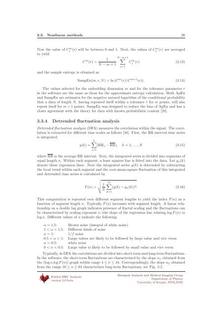
3.3. Nonlinear methods 26Now the value of Cj m(r) will be between 0 and 1. Next, the values of Cm j (r) are averagedto yieldN−m+1C m 1 ∑(r) =Cj m (r) (3.13)N − m +1and the sample entropy is obtained asj=1SampEn(m, r, N) =ln(C m (r)/C m+1 (r)). (3.14)The values selected for the embedding dimension m and for the tolerance parameter rin the software are the same as those for the approximate entropy calculation. Both ApEnand SampEn are estimates for the negative natural logarithm of the conditional probabilitythat a data of length N, having repeated itself within a tolerance r for m points, will alsorepeat itself for m + 1 points. SampEn was designed to reduce the bias of ApEn and has acloser agreement with the theory for data with known probabilistic content [20].3.3.4 Detrended fluctuation analysisDetrended fluctuation analysis (DFA) measures the correlation within the signal. The correlationis extracted for different time scales as follows [36]. First, the RR interval time seriesis integratedk∑y(k) = (RR j − RR), k =1,...,N (3.15)j=1where RR is the average RR interval. Next, the integrated series is divided into segments ofequal length n. Within each segment, a least squares line is fitted into the data. Let y n (k)denote these regression lines. Next the integrated series y(k) is detrended by subtractingthe local trend within each segment and the root-mean-square fluctuation of this integratedand detrended time series is calculated byF (n) = √ 1 N∑(y(k) − y n (k))N2 . (3.16)k=1This computation is repeated over different segment lengths to yield the index F (n) asafunction of segment length n. Typically F (n) increases with segment length. A linear relationshipon a double log graph indicates presence of fractal scaling and the fluctuations canbe characterized by scaling exponent α (the slope of the regression line relating log F (n) tolog n. Different values of α indicate the followingα =1.5: Brown noise (integral of white noise)1
3.3. Nonlinear methods 27−0.6−0.8log F(n)−1−1.2−1.4α 1α 2−1.6−1.80.6 0.8 1 1.2 1.4 1.6 1.8log nFigure 3.2: Detrended fluctuation analysis. A double log plot of the index F (n) as a functionof segment length n. α 1 and α 2 are the short term and long term fluctuation slopes,respectively.3.3.5 Correlation dimensionAnother method for measuring the complexity or strangeness of the time series is the correlationdimension which was proposed in [13]. The correlation dimension is expected to giveinformation on the minimum number of dynamic variables needed to model the underlyingsystem and it can be obtained as follows.Similarly as in the calculation of approximate and sample entropies, form length mvectors u ju j =(RR j , RR j+1 ,...,RR j+m−1 ), j =1, 2,...,N − m + 1 (3.17)and calculate the number of vectors u k for which d(u j ,u k ) ≤ r, thatisCj m (r) = nbr of { ∣u k d(uj ,u k ) ≤ r }N − m +1∀ k (3.18)where the distance function d(u j ,u k ) is now defined as∑d(u j ,u k )= √ m (u j (l) − u k (l)) 2 . (3.19)l=1Next, an average of the term C m j(r) istakenC m (r) =N−m+11 ∑N − m +1j=1C m j(r) (3.20)Kubios HRV Analysisversion 2.0 betaBiosignal Analysis and Medical Imaging GroupDepartment of PhysicsUniversity of Kuopio, FINLAND
- Page 3 and 4: 4.3.2 Report sheet . . . . . . . .
- Page 5 and 6: 1.1. System requirements 51.1 Syste
- Page 7: 1.2. Installation 74. Next, select
- Page 10 and 11: 1.2. Installation 1010. The MATLAB
- Page 12 and 13: 1.2. Installation 1214. When the in
- Page 14 and 15: 1.4. Software home page 14• Delet
- Page 16 and 17: Chapter 2Heart rate variabilityHear
- Page 18: 2.2. Derivation of HRV time series
- Page 21 and 22: 2.3. Preprocessing of HRV time seri
- Page 23 and 24: 3.2. Frequency-domain methods 23In
- Page 25: 3.3. Nonlinear methods 253.3.2 Appr
- Page 29 and 30: 3.3. Nonlinear methods 29987Time (m
- Page 31 and 32: 3.5. Summary of HRV parameters 31Ta
- Page 33 and 34: 4.1. Input data formats 33Figure 4.
- Page 35 and 36: 4.2. The user interface 35Figure 4.
- Page 37 and 38: 4.2. The user interface 37In additi
- Page 39 and 40: 4.2. The user interface 39Figure 4.
- Page 41 and 42: 4.2. The user interface 41Figure 4.
- Page 43 and 44: 4.3. Saving the results 431. Softwa
- Page 45 and 46: 4.3. Saving the results 45Figure 4.
- Page 47 and 48: 4.4. Setting up the preferences 47F
- Page 49 and 50: 4.4. Setting up the preferences 49F
- Page 51 and 52: Chapter 5Sample runsIn this chapter
- Page 53 and 54: 5.1. Sample run 1: General analysis
- Page 55 and 56: 5.1. Sample run 1: General analysis
- Page 57 and 58: 5.2. Sample run 2: Time-varying ana
- Page 59 and 60: Appendix AFrequently asked question
- Page 61 and 62: 61 Why do the power values of Kubio
- Page 63 and 64: References[1] V.X. Afonso. ECG QRS
- Page 65 and 66: References 65[28] J. Mateo and P. L
3.3. Nonlinear methods 26Now the value of Cj m(r) will be between 0 <strong>and</strong> 1. Next, the values of Cm j (r) are averagedto yieldN−m+1C m 1 ∑(r) =Cj m (r) (3.13)N − m +1<strong>and</strong> the sample entropy is obtained asj=1SampEn(m, r, N) =ln(C m (r)/C m+1 (r)). (3.14)The values selected for the embedding dimension m <strong>and</strong> for the tolerance parameter rin the software are the same as those for the approximate entropy calculation. Both ApEn<strong>and</strong> SampEn are estimates for the negative natural logarithm of the conditional probabilitythat a data of length N, having repeated itself within a tolerance r for m points, will alsorepeat itself for m + 1 points. SampEn was designed to reduce the bias of ApEn <strong>and</strong> has acloser agreement with the theory for data with known probabilistic content [20].3.3.4 Detrended fluctuation analysisDetrended fluctuation analysis (DFA) measures the correlation within the signal. The correlationis extracted for different time scales as follows [36]. First, the RR interval time seriesis integratedk∑y(k) = (RR j − RR), k =1,...,N (3.15)j=1where RR is the average RR interval. Next, the integrated series is divided into segments ofequal length n. Within each segment, a least squares line is fitted into the data. Let y n (k)denote these regression lines. Next the integrated series y(k) is detrended by subtractingthe local trend within each segment <strong>and</strong> the root-mean-square fluctuation of this integrated<strong>and</strong> detrended time series is calculated byF (n) = √ 1 N∑(y(k) − y n (k))N2 . (3.16)k=1This computation is repeated over different segment lengths to yield the index F (n) asafunction of segment length n. Typically F (n) increases with segment length. A linear relationshipon a double log graph indicates presence of fractal scaling <strong>and</strong> the fluctuations canbe characterized by scaling exponent α (the slope of the regression line relating log F (n) tolog n. Different values of α indicate the followingα =1.5: Brown noise (integral of white noise)1


