USER'S GUIDE - Biosignal Analysis and Medical Imaging Group

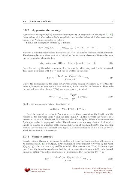
3.3. Nonlinear methods 253.3.2 Approximate entropyApproximate entropy (ApEn) measures the complexity or irregularity of the signal [12, 40].Large values of ApEn indicate high irregularity and smaller values of ApEn more regularsignal. The ApEn is computed as follows.First, a set of length m vectors u j is formedu j =(RR j , RR j+1 ,...,RR j+m−1 ), j =1, 2,...N − m +1 (3.7)where m is called the embedding dimension and N is the number of measured RR intervals.The distance between these vectors is defined as the maximum absolute difference betweenthe corresponding elements, i.e.,d(u j ,u k )=max { |RR j+n − RR k+n | ∣ ∣ n =0,...,m− 1}. (3.8)Next, for each u j the relative number of vectors u k for which d(u j ,u k ) ≤ r is calculated.This index is denoted with Cj m (r) andcanbewrittenintheformCj m (r) =nbr of { ∣u k d(uj ,u k ) ≤ r }∀ k. (3.9)N − m +1Due to the normalization, the value of Cj m (r) is always smaller or equal to 1. Note that thevalue is, however, at least 1/(N − m +1)sinceu j is also included in the count. Then, takethe natural logarithm of each Cj m (r) and average over j to yieldΦ m (r) =Finally, the approximate entropy is obtained asN−m+11 ∑ln Cj m (r). (3.10)N − m +1j=1ApEn(m, r, N) =Φ m (r) − Φ m+1 (r). (3.11)Thus, the value of the estimate ApEn depends on three parameters, the length m of thevectors u j , the tolerance value r, and the data length N. In this software the value of m isselected to be m = 2. The length N of the data also affects ApEn. When N is increased theApEn approaches its asymptotic value. The tolerance r has a strong effect on ApEn and itshould be selected as a fraction of the standard deviation of the data (SDNN). This selectionenables the comparison of different data types. A common selection for r is r =0.2SDNN,which is also used in this software.3.3.3 Sample entropySample entropy (SampEn) is similar to ApEn, but there are two important differences inits calculation [40, 20]. For ApEn, in the calculation of the number of vectors u k for whichd(u j ,u k ) ≤ r also the vector u j itself is included. This ensures that Cj m (r) is always largerthan 0 and the logarithm can be applied, but at the same time it makes ApEn to be biased.In sample entropy the self-comparison of u j is eliminated by calculating Cj m (r) asCj m (r) = nbr of { ∣u k d(u j ,u k ) ≤ r }∀ k ≠ j. (3.12)N − mKubios HRV Analysisversion 2.0 betaBiosignal Analysis and Medical Imaging GroupDepartment of PhysicsUniversity of Kuopio, FINLAND