USER'S GUIDE - Biosignal Analysis and Medical Imaging Group

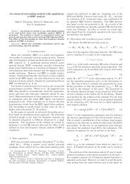
2.3. Preprocessing of HRV time series 20amount of artifact-free data is insufficient, proper interpolation methods can be used toreduce these artifacts, see, e.g., [21, 22, 29].Another common feature that can alter the analysis significantly are the slow linearor more complex trends within the analyzed time series. Such slow nonstationarities arecharacteristic for HRV signals and should be considered before the analysis. The origins ofnonstationarities in HRV are discussed, e.g., in [3]. Two kinds of methods have been usedto get around the nonstationarity problem. In [48], it was suggested that HRV data shouldbe systematically tested for nonstationarities and that only stationary segments should beanalyzed. Representativeness of these segments in comparison with the whole HRV signalwas, however, questioned in [14]. Other methods try to remove the slow nonstationary trendsfrom the HRV signal before analysis. The detrending is usually based on first order [23, 31]or higher order polynomial [39, 31] models. In addition, this software includes an advanceddetrending procedure originally presented in [43]. This approach is based on smoothnesspriors regularization.2.3.1 Smoothness priors based detrending approachLet z ∈ R N denote the RR interval time series which can be considered to consist of twocomponentsz = z stat + z trend (2.1)where z stat is the nearly stationary RR interval series of interest, z trend is the low frequencyaperiodic trend component, and N is the number of RR intervals. Suppose that the trendcomponent can be modeled with a linear observation model asz trend = Hθ + e (2.2)where H ∈ R N×p is the observation matrix, θ ∈ R p are the regression parameters, and e isthe observation error. The task is then to estimate the parameters by some fitting procedureso that ẑ trend = H ˆθ can be used as the estimate of the trend. The properties of the estimatedepend strongly on the properties of the basis vectors (columns of the matrix H) inthefitting. A widely used method for the solution of the estimate ˆθ is the least squares method.However, a more general approach for the estimation of ˆθ is used here. That is, the so-calledregularized least squares solution{ˆθ λ =argmin ‖z − Hθ‖ 2 + λ 2 ‖D d (Hθ)‖ 2} (2.3)θwhere λ is the regularization parameter and D d indicates the discrete approximation of thed’th derivative operator. This is clearly a modification of the ordinary least squares solutionto the direction in which the side norm ‖D d (Hθ)‖ gets smaller. In this way, prior informationabout the predicted trend Hθ can be implemented to the estimation. The solution of (2.3)canbewrittenintheformˆθ λ =(H T H + λ 2 H T D T d D dH) −1 H T z (2.4)and the estimate for the trend which is to be removed asẑ trend = H ˆθ λ . (2.5)The selection of the observation matrix H can be implemented according to some knownproperties of the data z. For example, a generic set of Gaussian shaped functions or sigmoidscan be used. Here, however, the trivial choice of identity matrix H = I ∈ R N×N is used. InKubios HRV Analysisversion 2.0 betaBiosignal Analysis and Medical Imaging GroupDepartment of PhysicsUniversity of Kuopio, FINLAND