Chapter 6: Time Series Analysis

ATM 552 Notes: Time Series Analysis - Section 6a Page 1036. Time (or Space) Series AnalysisIn this section we will consider some common aspects of time series analysisincluding autocorrelation, statistical prediction, harmonic analysis, power spectrum analysis,and cross-spectrum analysis. We will also consider space-time cross spectral analysis, acombination of time-Fourier and space-Fourier analysis, which is often used inmeteorology. The techniques of time series analysis described here are frequentlyencountered in all of geophysics and in many other fields.We will spend most of our time on classical Fourier spectral analysis, but willmention briefly other approaches such as Maximum Entropy (MEM), Singular SpectrumAnalysis (SSA) and the Multi-Taper Method (MTM). Although we include a discussion ofthe historical Lag-correlation spectral analysis method, we will focus primarily on the FastFourier Transform (FFT) approach. First a few basics6.1 Autocorrelation6.1.1 The Autocorrelation FunctionGiven a continuous function x(t), defined in the interval t 1 < t < t 2 , the autocovariancefunction ist 2 1 ( ) =t 2 t 1 x' t (6.1)where primes indicate deviations from the mean value, and we have assumed that >0. Inthe discrete case where x is defined at equally spaced points, k = 1,2,.., N, we can calculatethe autocovariance at lag L.( L) =1N 2LCopyright 2005 Dennis L. Hartmann 1/25/05 5:04 PM 103t 1N L x' k x' k + L = x' k x' k+ L ; L = 0, ±1, ±2,±3,... (6.2)k = LThe autocovariance is the covariance of a variable with itself (Greek autos = self) at someother time, measured by a time lag (or lead) . Note that ( 0) = x' 2 , so that theautocovariance at lag zero is just the variance of the variable.The Autocorrelation function is the normalized autocovariance function ()/(0) = r(); -1< r() < 1; r(0) = 1; if x is not periodic r() 0, as . It is normally assumed that datasets subjected to time series analysis are stationary . The term stationary time seriesnormally implies that the true mean of the variable and its higher-order statistical momentsare independent of the particular time in question. Therefore it is usually necessary toremove any trends in the time series before analysis. This also implies that theautocorrelation function can be assumed to be symmetric, () = (-). Under theassumption that the statistics of the data set are stationary in time, it would also bereasonable to extend the summation in (6.2) from k=L to N in the case of negative lags, and

ATM 552 Notes: Time Series Analysis - Section 6a Page 104from k=1 to N-L in the case of positive lags. Such an assumption of stationarity is inherentin much of what follows.6.1.2 Red Noise:We define a “red noise” time series as being of the form:x(t) = ax(t t) +(1 a 2 ) 1/2 (t) (6.3)where x is a standardized variablex = 0, x' 2 =1, a is on the interval between zero andone and measures the degree to which memory of previous states is retained (0 < a < 1), is a random number drawn from a standardized normal distribution, and t is the timeinterval between data points.Multiply (6.3) by x(t-t) and average to show that a is the one-lag autocorrelation, or theautocorrelation at one time step, t.xtt ( )xt ()= ax( t t)xtt( )+ ( 1 a 2 ) 1/2 xtt ( )= a 1 + ( 1 a 2 ) 1/2 0xtt ( )xt ()= r( t) = a; i.e., a is the autocorrelation at tProjecting into the future, we obtainxt+ ( t)= ax()+ t ( 1 a 2 ) 1/2 = a 2 xtt ( )+ a 1 a 2( ) 1/2 + ( 1 a 2 ) 1/2 = a 2 xtt ( )+ ( a +1) ( 1 a 2 ) 1/2 Now x(t+2t) = ax(t+t) + . Consistent with (6.2), multiply by x(t) and average using thedefinitions above.xt ()xt+ ( 2t) = ax( t + t)xt()+ x()tr( 2t)= ar( t) + 0r( 2t)= ( r( t)) 2or by inductionrnt ( ) = r n ( t)So for a red noise time series, the autocorrelation at a lag of n time steps is equal to theautocorrelation at one lag, raised to the power n. A function that has this property is theCopyright 2005 Dennis L. Hartmann 1/25/05 5:04 PM 104

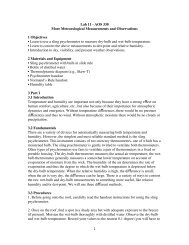
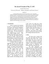
ATM 552 Notes: Time Series Analysis - Section 6a Page 105exponential function, e nx = ( e x ) n , so we may hypothesize that the autocorrelation functionfor red noise has an exponential shape.or if = nt,The autocorrelation function for red noise.rnt ( ) = exp{ nt T}.r( )= exp( T) where T = -t ln a (6.4)1.00.80.60.40.20.0-2 -1.5 -1 -0.5 0 0.5 1 1.5 2/TIn summary, if we are given a red noise time series, also called a Markov process,xt ()= ax( t t)+ ( 1 a 2 ) 1/2 (t) (6.5)then its autocorrelation function is,r( )= exp( T) (6.6)where the autocorrelation e-folding decay time is given by, T =-t ln aCopyright 2005 Dennis L. Hartmann 1/25/05 5:04 PM 105

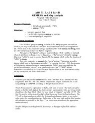
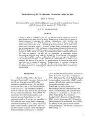
ATM 552 Notes: Time Series Analysis - Section 6a Page 106AmplitudeAmplitudeAmplitudeAmplitudeAmplitudeAmplitude210-1Periodic-20 0.5 1 1.5 2 2.5 32Time10-1Two Periods-20 0.5 1 1.5 2 2.5 32Time10-1White Noise-20 0.5 1 1.5 2 2.5 32Time10-1-20 0.5 1 1.5 2 2.5 3Time21Red Noise (0.8)+ Period0-1-20 0.5 1 1.5 2 2.5 32Time10-1Red NoiseSawtooth WaveCorrelationCorrelationCorrelationCorrelationCorrelationCorrelation1-20 -15 -10 -5 0 5 10 15 20Time Lag1-210 0.5 1 1.5 2 2.5 3 -20 -15 -10 -5 0 5 10 15 20TimeTime LagFigure. Comparison of time series and autocorrelation functions for various cases.0.5Copyright 2005 Dennis L. Hartmann 1/25/05 5:04 PM 10610.500.500.5PeriodicTwo Periods1-20 -15 -10 -5 0 5 10 15 20Time Lag10.500.5-0.50.5White Noise1-20 -15 -10 -5 0 5 10 15 20Time Lag10.500.50-0.5-110.50Red Noise (0.8)-1-20 -15 -10 -5 0 5 10 15 20Time Lag1Red Noise (0.8)+ Period-20 -15 -10 -5 0 5 10 15 20Time LagSawtooth Wave

ATM 552 Notes: Time Series Analysis - Section 6a Page 1076.1.3 Statistical Prediction and Red NoiseConsider a prediction equation of the formx ˆ ( t + t)= a' xt ()+ b' xtt ( ) (6.7)where x = 0 . a' and b' are chosen to minimize the rms error on dependent data. Recall fromour discussion of multiple regression that for two predictors x 1 and x 2 used to predict yrx ( 2 , y) rx ( 1 ,y)rx ( 1 ,x 2 )In the case where the equality holds, r(x 2 ,y) is equal to the “minimum useful correlation”discussed in Chapter 3 and will not improve the forecasting skill beyond the level possibleby using x 1 alone. In the case of trying to predict future values from prior times, r(x 2 ,y) =r(2t), and r(x 1 ,y) = r(x 1 ,x 2 ) = r(t) so that we must haver( 2t) > r( t) 2in order to justify using a second predictor at two time steps in the past. Note that for rednoiser( 2t) = r( t) 2so that the value at two lags previous to now always contributes exactly the minimum useful,and nearly automatic, correlation, and there is no point in using a second predictor if thevariable we are trying to predict is red noise. All we can use productively is the presentvalue and the autocorrelation function,xt+ ( t)= xt () with an R 2 = a 2 = r( t) 2This is just what is called a persistence forecast, we assume tomorrow will be like today.6.1.4 White NoiseIn the special case r(t) = a = 0, our time series is a series of random numbers,uncorrelated in time so that r() = (0) a delta function. For such a “white noise” timeseries, even the present value is of no help in projecting into the future. The probabilitydensity function we use is generally normally distributed about zero mean, and this isgenerated by the ‘randn’ function in Matlab.Copyright 2005 Dennis L. Hartmann 1/25/05 5:04 PM 107

ATM 552 Notes: Time Series Analysis - Section 6a Page 1086.1.5 Degrees of Freedom/Independent SamplesLeith [J. Appl. Meteor., 1973, p. 1066] has argued that for a time series of red noise,the number of independent samples N* is given byN* = Nt2T = total length of recordtwo times e - folding time of autocorrelation(6.9)where N is the number of data points in the time series, t is the time interval between datapoints and T is the time interval over which the autocorrelation drops to 1/e. In other words,the number of degrees of freedom we have is only half of the number of e-folding times ofdata we have. The more autocorrelated our data is in time, the fewer degrees of freedom weget from each observation.For Red Noise:thuse.g., for = tr( )= e T ln r( )T = -t/ln[r(t)], so thatT = ln( r( ))( ) = TN *N = 1 2ln[ r ( t ) ] ; N * 1 (6.10)NSample Values:r(t) < 0.16 0.3 0.5 0.7 0.9N*/N 1 0.6 0.35 0.18 0.053Leith’s formula (6.9) is consistent with Taylor(1921) for the case of a red noiseprocess. Taylor said thatN *N = 12L(6.11)Where L is given by,L = r( ') d '(6.12)0If we substitute the fomula for the autocorrelation function of red noise, (6.4) into 6.12),then we get that L=T, and Taylor’s formula is the same as Leith’s. You may see adimensional inconsistency in (6.11), but this disappears if you consider that Taylor is usingtime in nondimensional units of the time step, t’=t/t, ’=/t, so that L=T/ t.Copyright 2005 Dennis L. Hartmann 1/25/05 5:04 PM 108

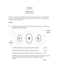
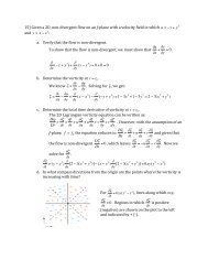
ATM 552 Notes: Time Series Analysis - Section 6a Page 109The factor of two comes into the bottom of the above expression for N* so that theintervening point is not easily predictable from the ones immediately before and after. Ifyou divide the time series into units of e-folding time of the auto-correlation, T, One canshow that, for a red noise process, the value at a midpoint, which is separated from its twoadjacent points by the time period T, can be predicted from the two adjoining values withcombined correlation coefficient of about 2e -1 , or about 0.52, so about 25% of the variancecan be explained at that point, and at all other points more can be explained. This may seema bit conservative.Indeed, Bretherton et al, (1999) suggest that, particularly for variance and covarianceanalysis a more accurate formula to use is:N *N =( 1 r(t)2 )( 1 + r(t) 2 )(6.13)If we compare the functional dependence of N*/N from Bretherton et al.(1999), formula(6.13) with that of Leith/Taylor from formula (6.10) we can make the plot below.1.21N*/N - Leith(1973)N*/N - Bretherton et al. (1999)0.8N*/N0.60.40.200 0.2 0.4 0.6 0.8 1So you can see that the Bretherton, et al. formula, which is appropriate for use in covarianceproblems, is more generous than Leith’s conservative formula, allowing about twice asmany degrees of freedom when the autocorrelation at one lag is large.r(∆t)References:Bretherton, C. S., M. Widmann, V. P. Dymnikov, J. M. Wallace and I. Blade, 1999: Theeffective number of spatial degrees of freedom of a time-varying field. J. Climate, 12,1990-2009.Copyright 2005 Dennis L. Hartmann 1/25/05 5:04 PM 109

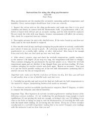
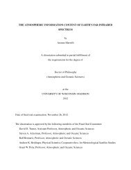
ATM 552 Notes: Time Series Analysis - Section 6a Page 110Leith, C. E., 1973: The standard error of time-averaged estimates of climatic means. J.Appl. Meteorol., 12, 1066-1069.Taylor, G. I., 1921: Diffusion by continuous movement. Proc. London Math. Soc., 21,196-212.6.1.6 Verification of Forecast ModelsConsider a forecast model that produces a large number of forecasts x f of x. Themean square (ms) error is given by( x x f ) 2The skill of the model is related to the ratio of the ms error to the variance of x about itsclimatological mean. Suppose that the model is able to reproduce climatological statistics inthe sense thatx f = x , x' f2 = x'2 .so thatIf the model has no skill thenx' x' f = 0( x x f ) 2 = ( x' x' f ) 2 = x' 2 2 2 x' x' f + x' f = 2x'2This result may seem somewhat paradoxical at first. Why is it not simply x' 2 ?The average root mean squared difference between two randomly chosen values with thesame mean is larger by 2' than that of each of these values about their common mean.21Two time Series with r(1)=0.70-1-20 50 100 150 200TimeThe following figure shows a plot of the rms error versus prediction time interval for ahypothetical forecast model whose skill deteriorates to zero as .Copyright 2005 Dennis L. Hartmann 1/25/05 5:04 PM 110

ATM 552 Notes: Time Series Analysis - Section 6a Page 111rmserror cFor > c the model appears to have no skill relative to climatology, yet it is clearthat it must still have some skill in an absolute sense since the error has not yet leveled off.The model can be made to produce a forecast superior to climatology if we use a regressionequation of the form.x ˆ f = ax f + ( 1 a)xLeast-squares regression to minimize( x x ˆ f ) 2yieldsa = x' x' fx' 2 The multiple correlation factor, R, for the original regressionSo we should choose a = R().As the skill of the prediction scheme approaches zero for large the ˆ x f forecast isweighted more and more heavily toward climatology and produces an error growth like thedotted curve in the figure above.Problem:Prove that at the point where the rms error of a simple forecast x f , passes the error ofclimatology (the average), where = c , a = 0.5, and at that point the rms error of x ˆ f equals0.87 times the rms error of x f .Copyright 2005 Dennis L. Hartmann 1/25/05 5:04 PM 111

ATM 552 Notes: Time Series Analysis - Section 6a Page 1126.2 Harmonic AnalysisHarmonic analysis is the interpretation of a time or space series as a summation ofcontributions from harmonic functions, each with a characteristic time or space scale.Consider that we have a set of N values of y(t i ) = y i . Then we can use a least-squaresprocedure to find the coefficients of the following expansionN2yt ( ) = A + A cos2k to k T + B sin2k t k T k =1(6.14)where T = the length of the period of record. y(t) is a continuous function of t which passesthrough all of the data points. Note that B k = 0 when k=N/2 , since you cannot determinethe phase of the wave with a wavelength of two time steps. If the data points are not evenlyspaced in time then we must be careful. The results can be very sensitive to small changesin y i . One should test for the effects of this sensitivity by imposing small variations in y iand be particularly careful where there are large gaps. Where the data are unevenly spacedit may be better to eliminate the higher harmonics. In this case one no longer achieves anexact fit, but the behavior may be much better between the data points.Useful Math Identities:It may be of use to you to have this reference list of trigonometric identities:cos( ) = cos cos + sin sin ; tan = sincos(6.15)You can use the above two relations to show that:C cos + S sin =( ) ; where A = C 2 + S 2 ; o = Arc tan S CA cos o(6.16)where you need to note the signs of S and C to get the phase in the correct quadrant.The complex forms of the trig functions also come up importantly here.Also, from this you can get;e i = cos + i sin where i = 1 (6.17)sin = ei e i2i; cos = ei + e i2(6.18)If you need more of these, check any book of standard mathematical tables.Copyright 2005 Dennis L. Hartmann 1/25/05 5:04 PM 112

ATM 552 Notes: Time Series Analysis - Section 6a Page 1136.2.1 Evenly Spaced Data Discrete Fourier TransformOn the interval 0 < t < T chosen such that t 1 =0 and t N+1 = T where N is an evennumber. The analytic functions are of the formcos( 2k it T),sin( 2k it T) (6.19)t is the (constant) spacing between the grid points. In the case of evenly spaced data wehave:a) a o = the average of y on interval 0

ATM 552 Notes: Time Series Analysis - Section 6a Page 114or, alternativelyN2 1yt ( ) = y + C k cos 2kk =1T( )t t kC k2 = Ak2 + Bk2 and tk = + A NtN 2 cos T T2k1Btan k A k (6.23)Of course, normally these formulas would be obtained analytically using the a prioriinformation that equally spaced data on a finite interval can be used to exactly calculate theFourier representation on that interval (assuming cyclic continuation ad infinitum in bothdirections).The fraction of the variance explained by a particular function is given byr 2 ( y, x k ) = x' k y'2x'2 k y'2= A k 2 + B 2 k2y' 2 ,for k =1,2,... N 2 12A N 2y' 2 for k = N 2(6.24)The variance explained by a particular k isC2 k2 for k =1,2, ... N 2 1; A 2N 2 for k = N 2 (6.25)6.2.2 The Power SpectrumThe plot of C k2 vs. k is called the power spectrum of y(t) - the frequency spectrumif t represents time and the wavenumber spectrum if t represents distance. Strictly speakingC k2 represents a line spectrum since it is defined only for integral values of k, whichcorrespond to particular frequencies or wavenumbers. If we are sampling a finite datarecord from a larger time series, then this line spectrum has serious drawbacks.1. Integral values of k do not have any special significance, but are simplydetermined by the length of the data record T, which is usually chosen on thebasis of what is available.k j = j tT , j = 0,1,2,... N 22. The individual spectral lines each contain only about 2 degrees of freedom,since N data points were used to determine a mean, N/2 amplitudes and N/2 - 1phases (a mean and N/2 variances). Hence, assuming a reasonable amount ofCopyright 2005 Dennis L. Hartmann 1/25/05 5:04 PM 114

ATM 552 Notes: Time Series Analysis - Section 6a Page 115noise is present, a line spectrum may (should) have very poor reproducibilityfrom one finite sampling interval to another; even if the series is stationary(i.e., its true properties do not change in time). To obtain reproducible,statistically significant results we need to obtain spectral estimates with manydegrees of freedom.3. With the notable exceptions of the annual and diurnal cycles and their higherharmonics, most interesting “signals” in geophysical data are not trulyperiodic but only quasi-periodic in character, and are thus better representedby spectral bands of finite width, rather than by spectral lines.Continuous Power Spectrum: (k)All of the above considerations suggest the utility of a continuous power spectrumwhich represents the variance of y i (t) per unit frequency (or wavenumber) interval such thaty' 2 k*= ( k)dk (6.26)0So that the variance contributed is equal to the area under the curve (k), as shown below. kkk1 2k*kk* corresponds to one cycle per 2t, the highest frequency in y(t) that can be resolved withthe given spacing of the data points. This k* is called the Nyquist frequency. If higherfrequencies are present in the data set they will be aliased into lower frequencies.0 k k*Copyright 2005 Dennis L. Hartmann 1/25/05 5:04 PM 115

ATM 552 Notes: Time Series Analysis - Section 6a Page 116•tt•ttrue periodt = 2/3 t•aliased periodt = 2.0ttrue wavenumber aliased wavenumberk = 3.0k * k = 1.0k *This is a problem when there is a comparatively large amount of variance beyond k * .Degrees of Freedom—Resolution Tradeoff:For a fixed length of record, we must balance the number of degrees of freedom foreach spectral estimate against the resolution of our spectrum. We increase the degrees offreedom by increasing the bandwidth of our estimates. Smoothing the spectrum means thatwe have fewer independent estimates but greater statistical confidence in the estimate weretain.High resolutionLower resolutionHigh Information Smooth/Average Lower InformationLow QualityHigh quality in a statisticalsense"Always" insist on adequate quality or you could make a fool of yourself.The number of degrees of freedom per spectral estimate is given by N/M* where M*is the number of independent spectral estimates and N is the actual number of data pointsy i (t) regardless of what the autocorrelation is. As long as we use a red-noise fit to thespectrum as our null hypothesis, we don’t need to reduce the number of degrees of freedomto account for autocorrelation.Copyright 2005 Dennis L. Hartmann 1/25/05 5:04 PM 116

ATM 552 Notes: Time Series Analysis - Section 6a Page 1176.2.3 Methods of Computing Power SpectraDirect Method:The direct method consists of simply performing a Fourier transform or regressionharmonic analysis of y i (t) to obtain C k2 . This has become economical because of the FastFourier Transform (FFT). Because the transform assumes cyclic continuity, it is desirableto "taper" the ends of the time series y i (t), as will be discussed in section 6.2.5. When wedo a Fourier analysis we get estimates of the power spectrum at N/2 frequencies, but eachspectral estimate has only two degrees of freedom. A spectrum with so few degrees offreedom is unlikely to be reproducible, so we want to find ways to increase the reliability ofeach spectral estimate, which is equivalent to a search for ways to increase the number ofdegrees of freedom of each estimate.How to obtain more degrees of freedom:a.) Average adjacent spectral estimates together. Suppose we have a 900 dayrecord. If we do a Fourier analysis then the bandwidth will be 1/900 day -1 ,and each of the 450 spectral estimates will have 2 degrees of freedom. If weaveraged each 10 adjacent estimates together, then the bandwidth will be 1/90day -1 and each estimate will have 20 d.o.f.b.) Average realizations of the spectra together. Suppose we have 10 time series of900 days. If we compute spectra for each of these and then average theindividual spectral estimates for each frequency over the sample of 10 spectra,then we can derive a spectrum with a bandwidth of 1/900 days -1 where eachspectral estimate has 20 degrees of freedom.So how do we estimate the degrees of freedom in the direct – FFT method? If wehave N data points, and the resulting spectrum provides a variance at N/2 frequencies, wehave two degrees of freedom per spectral estimate. If we smooth the spectrum, then wemust estimate the effect of this smoothing on the degrees of freedom, which would beincreased. If we average adjacent spectral estimates together, then we could assume that thenumber of degrees of freedom are doubled. In general, a formula would bed.o.f = N M *Where N is the total number of data points used to compute the spectrum estimate, and M*is the total number of degrees of freedom in the spectrum. For example, if you used 1024data points to estimate a spectrum with 64 independent spectral estiamtes, then the numberof degrees of freedom would be 1024/64 = 16.Lag Correlation Method:According to a theorem by Norbert Wiener, that we will illustrate below, theautocovariance (or autocorrelation, if we normalize) and the power spectrum are Fouriertransforms of each other. So we can obtain the power spectrum by performing harmonicCopyright 2005 Dennis L. Hartmann 1/25/05 5:04 PM 117

ATM 552 Notes: Time Series Analysis - Section 6a Page 118analysis on the lag correlation function on the interval -T L T L . The resulting spectrumcan be smoothed, or the number of lags can be chosen to achieve the desired frequencyresolution. The Fourier transform pair of the continuous spectrum and the continuous lagcorrelation are shown below.T L( k) = r( )e ik dT Lr( )= 12k *k *( k)e ik dk(6.27)The maximum number of lags L determines the bandwidth of the spectrum and the numberof degrees of freedom associated with each one. The bandwidth is 1 cycle/2T L , andfrequencies 0, 1 cycle/2T L , 2/2T L, 3/2T L, ..., 1/2t. There are12t1=T Lt2T L(6.28)of these estimates. Each withT L tN1 = N Ldegrees of freedom. (6.29)The lag correlation method is rarely used nowadays, because Fast Fourier Transformalgorithms are more efficient and widespread. The lag correlation method is important forintellectual and historical reasons, and because it comes up again if you undertake higherorder spectral analysis.Copyright 2005 Dennis L. Hartmann 1/25/05 5:04 PM 118