Fundamentals of scanning probe microscopy

Chapter 1. The scanning probe microscopy techniquereal time, so that when the tip is moved to a point x,y over the sample, the signal V(x,y) fed to thetransducer is proportional to the local departure of the sample surface from the ideal planeX,Y(z = 0). This makes possible to use the values V(x,y) to map the surface topography, ad toobtain an SPM image. During scanning the tip first moves above the sample along a certain line(line scan), thus the value of the signal fed to the transducer, proportional to the height value in thesurface topography, is recorded in the computer memory. Then the tip comes back to the initialpoint and steps to the next scanning line (frame scan), and the process repeats again. The feedbacksignal recorded during scanning is processed by the computer, and then the SPM surfacetopography image Z = f (x,y) is plotted by means of computer graphics. Alongside withinvestigation of the sample topography, probe microscopes allow to study various properties of asurface: mechanical, electric, magnetic, optical and many others.1.2. Scanning elements (scanners)It is necessary to control the working tip-sample distance and to move the tip over the samplesurface with high accuracy (at a level of Angstrom fractions) in order to make the probemicroscopes properly working. This problem is solved with the help of special transducers, orscanning elements (scanners). The probe microscope scanners are made of piezoelectric materials.Piezoelectric materials change their sizes in an external electric field. The inverse piezoeffectequation for crystals is as follows:u = d E ,ijijkkwhere u is the deformation tensor, are the electric field components, d are the componentsijEkof piezoelectric tensor. The piezoelectric coefficients are defined by the type of crystal symmetry.ijkTransducers made from piezoceramic materials are widely used in various technical applications.The piezoceramics is polarized polycrystalline material obtained by powder sintering from crystalferroelectrics. Polarization of ceramics is performed as follows. The ceramic is heated up above itsCurie temperature T c (for the majority of piezoceramics T c

Fundamentals of the scanning probe microscopyrPE rxFig. 2. Piezoceramic plate in an external electric fieldTubular piezoelements (Fig. 3) are widely used in scanning probe microscopy. They allowobtaining large enough movements with rather small control voltages. Tubular piezoelements arehollow thin-walled cylinders with electrodes (thin metal layers), plated on the external and internaltube surfaces, and the end tube faces remain uncovered.rxFig. 3. Tubular piezoelementUnder the influence of a potential difference between internal and external electrodes the tubechanges its length. The relative longitudinal deformation under the influence of a radial electricfield can be written as:u∆x= = dlxx ⊥E r0,where l 0is the length of the unstressed tube. The absolute lengthening of the piezo-tube is :l0x = d⊥Vh∆ ,where h is the thickness of the tube wall, V is the potential difference between internal and externalelectrodes. Thus, for the same applied voltage, the tube lengthening will be larger, for longer andthinner tubes.Assembly of three tubes into one unit (Fig. 4) allows to produce precise movements in threemutually perpendicular directions. Such scanning element is referred to as tripod.8

Chapter 1. The scanning probe microscopy techniqueYXZFig. 4. Scanning element as tripod, assembled on tubular piezoelementsThe drawbacks of such scanner are the complexity of manufacturing and the strong asymmetry ofits structure. Today the scanners made of one tubular element are most widely used in scanningprobe microscopy. The structure of a tubular scanner and the arrangement of electrodes arepresented in Fig. 5. The polarization vector is radially directed.P-Y+X Z-X+YFig. 5. Tubular piezo-scannerThe internal electrode is usually continuous. The external electrode is divided by cylindergeneratrixes into four sections. When differential-mode voltage is applied on opposite sections ofthe external electrode (with respect to the internal electrode) part of the tube reduces in length(where the field direction coincides with the polarization direction), and increases (where field andpolarization directions are opposite). This leads to a bend of the tube. Scanning in the X,Y plane isdone in this manner. Change of the internal electrode potential with respect to all external sectionsresults in lengthening or reduction of the tube along Z axis. Thus, it is possible to implement thethree-coordinate scanner on the basis of one piezo-tube. Real scanning elements frequently have amore complex structure; however the working principle remain the same.Scanners based on bimorph cells are also widely used. Bimorph is made of two plates ofpiezoelectric material, which have been glued together with opposite polarization vectors as shownin Fig. 6. If a voltage is applied to bimorph electrodes, as shown on Fig. 6, one of the plates will9

Fundamentals of the scanning probe microscopyextend, and the other one will be compressed, resulting in a bend of the whole element. In realconstructions of bimorph elements the potential difference between the internal common electrodeand external electrodes is created so that in one element the field coincides with the direction of apolarization vector, and in another element it is oppositely directed.EPFig. 6. Structure of a bimorph cellThe bimorph bending under the influence of electric fields is the working mechanism of bimorphpiezo-scanners. Combining three bimorph elements in one device makes possible to implement atripod (Fig. 7).BimorphelementXYZFig. 7. Three-coordinate scanner made of three bimorph elementsIf external electrodes of a bimorph element are divided into four sectors, then it is possible to movea stem (e.g. holding a tip) along the Z axis and in the X, Y plane using a single bimorph element(Fig. 8).10

Chapter 1. The scanning probe microscopy technique++__(a)+_(c)(b)(d)Fig. 8. Schematic representation of a bimorph piezo-scanner working mechanismIndeed, applying a differential-mode voltage on opposite pairs of external electrodes sections makesbending the bimorph so that the tip will move in the X,Y plane (Fig. 8 (a, b)). On the other hand, apotential applied to the internal electrode with respect to all sections of external electrodes makesbending the bimorph, so that the tip moves in the Z axis direction (Fig. 8 (c, d)).Piezoceramics nonlinearityDespite of a number of technological advantages over crystals, piezoceramics have somedrawbacks. One is the nonlinearity of piezoelectric properties. The dependence of the piezo-tubeshift size in Z direction on the value of the applied field is schematically shown in Fig. 9 as anexample. Generally (especially at large control fields) the piezoceramics are characterized bynonlinear dependence of the deformation on the field (i.e. on the control voltage). Thus,deformation of piezoceramics is a complex function of the applied electric field:ru = u ( E ).ijijFor small control fields the given dependence can be represented in the following way:u= d E + α E E ....,ij ijk k ijkl k l+where d ijk and α ijkl are the first and second order piezoelectric coefficients, respectively.11

Fundamentals of the scanning probe microscopyV∆ZZEE*Fig. 9. Schematic representation of dependenceof ceramics shift on the size of applied electric fieldTypical values of fields E*, at which nonlinear effects cannot be neglected, are about 100 V/mm.Therefore in scanning elements the control fields are usually kept small (within the linear rangeE

Chapter 1. The scanning probe microscopy techniquePiezoceramics hysteresisAnother drawback of piezoceramics is the presence of hysteresis in the transfer function ∆Z = f(V) ,i.e. the piezoceramic deformation depends on the sign of previously applied electric field.V∆ZZVFig. 11. Dependence of the piezo-tube shift on thevalue and direction of the applied voltageIn other words the piezoceramic shift ∆Z describes, in the (∆Z, V) plane, a looped trajectory wheredifferent ∆Z values are taken, depending on the time derivative of the control voltage V (Fig. 11).To avoid distortions in the SPM images caused by piezoceramics hysteresis, information is stored,in a sample scanning, only while tracing one of the loop branches ∆Z = f (V ).1.3. Devices for precise control of tip and sample positionsOne of the important technical requirements in scanning probe microscopy is the precision ofmovements of tip and sample, aiming at an accurate selection of the sampled area. Several types ofdevices performing movements of objects with high accuracy are used to solve this problem.Various mechanical reducers, in which coarse movements are converted into fine movements,became widely spread. For example lever devices, in which the reduction of movement is producedby the different length of the lever arms, are widely applied. The lever reducer is schematicallypresented in Fig. 12.∆LLl∆lFig. 12. Lever movement reducer schematic13

Fundamentals of the scanning probe microscopyThe mechanical lever downscales the movement by the following factor:∆LR =∆lLl= .Thus, the larger is the ratio between the arm L to the arm l, the more precisely the process of tip tosample approach can be controlled.Spring/cantilever reducers are also widely used in constructions of microscopes, in which themovements are scaled down exploiting the difference in stiffness of two elastic elements in series(Fig. 13). The structure usually consists of a rigid base, a spring and an elastic beam (cantilever).The elastic constant of the spring k and of the cantilever K are selected so that the condition k < Kis satisfied.kK∆l∆LFig. 13. Schematic of spring/cantilever movements reducerFrom the equilibrium condition it follows, thatF elast= k ⋅ ∆l= K ⋅ ∆L,where ∆l and ∆L are the spring and cantilever displacements, respectively. In this case the reductioncoefficient equals the ratio between the elastic constant of the elastic elements:∆lR =∆LKk= .Thus, the larger is the cantilever stiffness with respect to the spring stiffness, the more precisely it ispossible to control the displacement of the cantilever end.Stepping motorsStepping motors (SM) are electromechanical actuators, which transform electric pulses into discretemechanical movements (rotations). The important advantage of stepping motors is that they providea reliable correspondence between the angular displacement of the rotor and the number ofactuating current pulses. In SM the torque is created by magnetic coupling between the stator and14

Chapter 1. The scanning probe microscopy techniquethe rotor poles. The stator has several poles, made of high magnetic permeability material andassembled from separate plates to reduce the losses by eddy currents. The torque is proportional tothe magnetic field value, which is proportional to the current and to the number of coils. If thecurrent in one of the windings is switched on, the rotor takes a certain position. By switching off thecurrent in that winding and switching it on in another one, it is possible to move the rotor to the nextposition, etc. Thus, controlling the current in windings, it is possible to rotate the SM rotor in a stepby-stepmode. It will remain in the position set by the last switched on winding until the externalapplied torque does not exceed a threshold value called the holding torque. With higher appliedtorque the rotor will turn and try to take one of the following equilibrium positions.The simplest structure of a stepping motor is schematically shown in Fig. 14. It consists of a statorwith windings and a rotor with permanent magnets. The rotor poles have rectangular shape parallelto the motor axis. The motor shown in figure has 3 pairs of rotor poles and 2 pairs of stator poles.The stator has 2 independent windings, each one wound up on two opposite poles. The motorshown in Fig. 14 has an incremental step of 30 grad. When the current is switched on in one of thewindings, the rotor tends to take the position at which the unlike poles of rotor and stator areopposite to each other. To produce the continuous rotation it is necessary to switch on the windingsalternatively by applying a sequence of current pulses.Stator poles1Stator windingsNRotor poles2S1230ºSwitched on windingFig. 14. Stepping motor with permanent magnet rotorStepping motors having more complex structure and providing from 100 to 400 steps per revolution(incremental step from 3.6 to 0.9 degrees) are used in practice. If such motor drives a threaded axiswith a pitch of 1 mm, then an accuracy in object positioning better than 1 micron may be obtained.Additional mechanical reducers are applied to increase the accuracy. The possibility of electriccontrol allows the use stepping motors in automated systems to approach a tip to a sample inscanning probe microscopes.Step-by-step piezoelectric motorsRequirements of good insulation from external vibrations and necessity of working under vacuumimpose serious restrictions on application of mechanical devices for tip and sample movements. Inthis respect, devices based on piezoelectric converters, allowing to perform remote control ofobjects movement, became widely used in probe microscopes.15

Fundamentals of the scanning probe microscopyOne of the devices used for this purpose is the step-by-step inertial piezo-motor presented inFig. 15. This device includes the base (1) on which the piezoelectric tube (2) is fixed. The tube haselectrodes (3) on external and internal surfaces. The split spring (4) holds a cylinder with polishedsurface, massive enough (5) that supports the object to be moved. The moved object can be fixed tothe cylinder with the help of a spring or a captive nut that allows the device to work at anyorientation in space.453211. – base;2. – piezoelectric tube;3. – electrodes;4. – split spring;5. – cylindrical object holderFig. 15. – Step-by-step piezoelectric motorThe device works as follows. To move the object holder in the Z axis direction a saw tooth voltagesignal is applied to electrodes of the piezo-tube. The characteristic form of a control voltage pulse ispresented on Fig. 16.UFig. 16. Control voltage pulse form of a step-by-step inertial piezoelectric motorThe tube is smoothly extended or compressed (depending on the voltage polarity), and at the rampend, the object holder is shifted of the following amount:l = d31lUh∆ .At the end of the voltage ramp the tube returns suddenly to the starting position with an accelerationa , which has its maximal value in the beginning:t16

Chapter 1. The scanning probe microscopy technique2a = ∆lω ,where ω is the resonant frequency of longitudinal oscillations of the tube. If the followingcondition is satisfied :F fr< mamF( is the weight of the object holder, the friction force between the object holder and the splitfrspring) then the object holder, due to its inertia, slides relatively to the split spring. As a result, theobject holder makes a step K∆ l with respect to the starting position. The K factor depends on thecylinder weight and on the stiffness of the split spring. When the polarity of the control voltagepulses is reversed, the object movement direction changes. Thus, applying a saw tooth voltage ofvarious polarities to the piezo-tube electrodes, it is possible to move the object in space and toapproach the tip to the sample in a scanning probe microscope.1.4. Protection of SPM against external influencesProtection against vibrationsAny scanning probe microscope is an oscillatory system with its own resonant frequencies ωk.External mechanical vibrations with frequencies coinciding with ωk, may excite resonance in themeasuring heads structure, which results in fluctuations of the tip relatively to the sample that isperceived as a parasitic periodic noise deforming and dithering the SPM images of samples surface.To reduce the influence of external vibrations the measuring heads are made of massive metaldetails with high (more than 100 kHz) resonant frequencies. Scanners have low resonantfrequencies. In the design of modern SPM it is necessary to reach a compromise between thescanner range (the size of maximum scanned area) and its resonant frequency. Typical values forresonant frequencies are in the range 10 - 100 kHz.Various types of vibration-insulating systems can be distinguished as passive and active ones. Thebasic idea incorporated in passive vibration-insulating systems is the following. The amplitude offorced oscillations of a mechanical system quickly decays at large values of the difference betweenthe excitation frequency and own resonant frequency of the system (see Fig. 17).AA 0ωω 0ω extFig. 17. Blue color: SPM resonant curveRed color : frequency spectrum of external vibrations17

Fundamentals of the scanning probe microscopyω >> ωTherefore external vibrations with frequenciesext 0practically do not affect the oscillatorysystem. Hence, if the measuring head of a probe microscope is placed on a vibration-insulatingplatform or on an elastic suspension (Fig. 18), then only external fluctuations with frequencies closeto the resonant frequency of the vibration-insulating system will be picked-up by the microscope.Since the resonant frequencies of SPM heads are in the range 10 - 100 kHz, choosing the resonantfrequency of vibration-insulating systems low enough (about 5 - 10 Hz), it is possible to protect thedevice from external vibrations rather effectively. In order to quench oscillations even at their ownresonant frequencies, dissipative elements with viscous friction are introduced into vibrationinsulatingsystems.Fig. 18. Passive vibration- insulating systemsThus, to reach effective protection it is necessary to make the resonant frequency of the vibrationinsulatingsystem as small as possible. However, it is difficult to realize in practice very lowfrequencies. For spring platforms and elastic suspensions the resonant frequency iskω0= ,mwhere k is the spring (or suspension) elastic constant, m the weight of the vibration-insulatingplatform together with the SPM head. We shall estimate parameters of the vibration-insulatingsystem providing suppression of high-frequency vibrations. From the equilibrium condition itfollows, thatmg= k∆l,∆ l is the lengthening (or compression) of the elastic element, g is the gravitationalwhereacceleration. Then, for the size of lengthening:gm g g∆ l = = = ≅ 0.25 ⋅k ω2p122( 2πν) ν.Thus, in order to obtain for the vibration-insulating system a resonant frequency smaller than 1 Hz,the lengthening (or compression) of the elastic element must be more than 25 cm. Such lengtheningcan be obtained in the simplest way using springs or rubber suspensions. Taking into account, that18

Chapter 1. The scanning probe microscopy techniquethe relative stretching of springs can reach 100 %, the length of the suspension elastic element maybe 25 cm, and, hence, the total size of the vibration-isolating system will be 50 cm. If resonantfrequency requirements are less stringent, it is possible a substantial reduction of the of thevibration-insulating system size. So, for a frequency cut-off of 10 Hz the compression should beonly 2,5 mm. Such compression is may be easily obtained using a stack of metal plates with rubberspacers, which considerably reduces the dimensions of the system.Active systems for suppression of external vibrations are also successfully used to protect the SPMheads. Such devices are electromechanical systems with a negative feedback, which stabilizes thevibration-insulating platform (Fig. 19).Vibration sensorSPMPlatformPiezoelectricsupportsFSBaseFig. 19. Active vibration-insulating system schematicThe working principle of active systems is the following. The vibration sensor (accelerometer)installed on the platform produces a signal that is fed to the feedback system (FS) where it isinverted, amplified and transmitted to the piezoelectric actuators, placed under the platform legs,canceling the platform acceleration. This is the so-called proportional adjustment. In fact, let theplatform oscillate with the frequency ⎤ under the action of external force, with amplitude u:u= u sin( ωt).0Then the platform acceleration is2u&= −ω u 0& .sin( ωt)The feedback system provides an antiphase signal = −a sin( ωt) to the supports; therefore theplatform displacement is due the superposition of two excitations:u fu= u = ( u0− a )sin( ωt)0.The feedback system will adjust the amplitude of the signal fed to the actuators until the platformacceleration reaches zero:u&& .=02−ω ( u − a )sin( ωt)Multistage constructions of vibration-insulating systems of various types are commonly used,allowing to increase the degree of protection of devices against external vibrations.19

Fundamentals of the scanning probe microscopyProtection against acoustic noiseAnother source of vibrations in the probe microscopes structure are acoustic noises of variousnature.Fig. 20. SPM protection against acoustic noiseAcoustic waves directly affect elements of SPM heads, resulting in oscillations of the tip withrespect to the sample surface. Various protective enclosures, allowing a sensible reduction of thelevel of acoustic noise are used to protect the SPM. The most effective protection against acousticnoise is to place the measuring head into a vacuum chamber.Reduction of the thermal drift of the tip position above the surfaceOne of important problems in the SPM is the stabilization of the tip position above the samplesurface. The main source of tip instability is the change of the room temperature or the warming upof SPM elements during operation. Temperature change of a body results in thermo elasticdeformations:uik= α ∆T,ikwhere uikis the deformations tensor, αikare the components of thermal expansion tensor,the temperature increment. For isotropic materials the thermal expansion coefficient is a scalar:α = α ⋅ ,ikδ ikδikis the ordinary Kronecker tensor, α is the thermal expansion coefficient. Absolutewherelengthening of microscope construction elements can be estimated from the following equations:∆Tisu∆l= = α ⋅ ∆T ;l0∆l= l α ⋅ ∆T0.20

Chapter 1. The scanning probe microscopy techniqueTypical values of expansion coefficients are in the rang 10 -5 – 10 -6 K -1 . Thus, heating a 10 cm longbody by 1°C its length increases on about 1 micron. Such deformations affect substantially the SPMperformance. To reduce the thermal drift, thermoregulation of SPM heads is used, or temperaturecompensatingelements are introduced in the head structure. The idea of temperature-compensationconsists in the following. Any SPM model can be schematized as a set of elements with differentthermal expansion coefficients (Fig. 21 (а)).l1l2l3l4l5ZYX(a)(b)Fig. 21. Compensation of thermal expansions in SPMIn order to reduce the thermal drift in the SPM measuring heads, compensating elements withdifferent expansion coefficients are introduced, in a geometry that brings to zero the sum oftemperature expansions in various parts of the structure:∑∑∆L = ∆l= ∆Tα l ⇒ 0 .iiii iThe simplest way to reduce the thermal drifts is to introduce in the SPM construction compensatingelements made of the same material and with the same characteristic sizes, as the basic elements ofthe SPM head (Fig. 21 (b)). When the temperature of such arrangement changes, the shift of the tipin Z direction is minimal. The measuring head of microscopes are axial-symmetric designed tostabilize the position of the tip in the X, Y plane.1.5. Acquisition and processing of SPM imagesScanning a surface in a SPM is like moving an electronic beam on the screen in the cathode raytube of a TV. The tip goes along a (row) first in forward, and then in the reverse direction(horizontal scanning), then passes to the next line (frame scanning). Movement of the tip is done insmall steps by the scanner that is driven by a saw tooth voltage produced by digital-to-analogconverters. The surface topographic information is stored, as a rule, during the forward pass.21

Fundamentals of the scanning probe microscopyjiFig. 22. Schematic illustration of the scanning process.The direction of the forward motion of the scanner is indicated by red arrowsReverse motion of the scanner is indicated by dark blue arrowsRegistration of the information is made in points on direct passThe information collected by the scanning probe microscope, is stored as a two-dimensional file ofinteger numbers (matrix). The physical meaning of these numbers is determined by the kind ofa ijinteraction, which was measured during scanning. To each value of ij pair of indexes corresponds acertain point of a surface within the scanning area. Coordinates of points of the sampled area arecalculated simply multiplying the corresponding index by the value of the distance between points:x i= x 0⋅ i , y ⋅ j .y j= 0Here x 0 and y 0 are the distances between adjacent points, along X and Y axes, where theinformation was recorded. As a rule, the SPM frames are square matrixes (whose size is commonly256×256 or 512×512 elements). Visualization of the SPM frame is done by computer graphics,basically, as three-dimensional (3D) or two-dimensional brightness (2D) images. At 3Dvisualization the image of a surface Z = f(x,y), is plotted in an axonometric view by pixels or lines.In addition to this, various ways of pixels brightening corresponding to various height of the surfacetopography are used. The most effective way of 3D images coloring is obtained simulating thesurface illumination by a point source located in some point of space above the surface (Fig. 23).Thus it is possible to emphasize small-scale topography inequalities. Same graphical instrumentsand computer processing are used for scaling and rotation of 3D SPM images. In 2D visualization(also named ″Top View″ image) to each point of the surface Z = f(x,y) is assigned a color (or abrightness) that corresponds to its z-value according to a given color-scale (or gray-scale). As anexample, the 2D image of a surface area is presented on Fig. 24.22

Chapter 1. The scanning probe microscopy techniqueFig. 23. 3D visualization of a surface topography with illumination on height (a)and with lateral illumination (b)Fig. 24. 2D brightness image of a surface topographyThe physical meaning of SPM images depend on the parameter that is used in the feedback loop.For example, the values stored in the Z = f(x,y) matrix may depend on the electric current valueflowing through the tip-surface contact with constant applied voltage, or they may depend on themain tip-surface interactive force (electric, magnetic, etc.). Besides these “maps” of the tip-sampleinteraction over the scanned area, a different type of information may be retrieved using SPM. Forexample, on a single point of the sample surface we may collect the dependence of the tunnelingcurrent on the applied voltage, the dependence of the interactive force on the tip-sample distance,etc. This information is stored as vector files or as matrixes of 2×N dimension, that may bedisplayed or printed using a set of standard tools for graphic presentation provided by the SPMsoftware. SPM images, alongside with the helpful information, contain also a lot of secondaryinformation affecting the data and appearing as image distortions. Possible distortions in SPMimages caused by imperfection of the equipment and by external parasitic influences areschematically presented on Fig. 25.23

Fundamentals of the scanning probe microscopyConstantcomponentHardwarenoisesConstantinclinationValid signalInstability oftip-sample contactScannerimperfectionNoise due to externalvibrationsFig. 25. Possible distortions in the SPM imagesSubtraction of a constant componentAs a rule, the SPM images contain a constant component, which does not bear useful informationabout the surface topography, but reflects the accuracy of sample approaching into the center of thedynamic range of scanner movement along the Z axis. The constant component is removed from theSPM frame using software tools so the new values of the topography heights in the frameare equal toZ'ij1= Z − Z , where Z =ij2 ∑N ijZ ij.Subtraction of a constant inclinationSurface images acquired using probe microscopes, as a rule, show inclination. It can be due toseveral reasons. First, the inclination may appear as a result of a tilted installation of the sampleonto the scanner or due to non-flatness of the sample; second, it might be connected with atemperature drift, which results in tip shifting with respect to the sample; third, it might be due to anon-linearity of the piezo-scanner movement. Inclined images take a large portion of Z-axis, so thatthe small image details become not visible. To eliminate this inconvenience, a subtraction of theconstant inclination is usually performed. For this purpose at the first stage the method of leastsquares is used to find an approximating plane P ( 1 ) ( x,y ), which has minimal deviations from thesurface topography Z = f(x,y) ( Fig. 26). Then the best-fit plane is subtracted from the SPM image.It is reasonable to subtract in various ways, depending on the inclination nature. If the inclination inthe SPM image is caused by sample tilt relative to the tip axis, we may rotate the plane by an anglecorresponding to the angle between the axis n r orthogonal to the best-fit plane and the Z axis; thusthe coordinates of the surface Z = f(x,y) will be transformed according to such rotation. However,this transformation may give a multiple-valued function Z = f(x,y). If the inclination is caused by a24

Chapter 1. The scanning probe microscopy techniquethermal drift, the procedure of inclination subtraction affects only the Z-coordinates of the SPMimage:Z'ij= Z − P .ij( 1 )ijThis allows to keep correct geometrical relations in the X,Y plane between objects in theSPM image.ZZn rYYXXFig. 26. Inclined plane interpolating the SPM imageFinally, an array with a smaller range of Z-values is obtained, and fine details of the image will bedisplayed with much larger contrast, becoming more visible.The result of plane subtraction from a real AFM image is presented on Fig. 27.Fig. 27. Subtraction of an inclined plane from AFM image25

Fundamentals of the scanning probe microscopyElimination of the distortions due to scanner imperfectionImperfection of the piezo-scanner properties leads to artifacts in the SPM image. The scannerimperfections, such as hysteresis (differences in direct and reverse motions), creep and nonlinearitymay be partially compensated by the hardware and by selection of optimum modes of scanning. Inany case the SPM images contain residual distortions, which are difficult to remove on thehardware level. In particular, since the scanner movement in X and Y directions affects the tip –sample distance (z-axis), the SPM images represent a superposition of the actual topography andsome surface of the second (and sometimes higher) order (Fig. 28).ZZYYXXFig. 28. Subtraction of a surface of the second order from the SPM imageThe approximating surface of the second order P (2) (x,y) is calculated using the least-squaresmethod, The fitting surface (with minimal deviations from the topographic surface Z = f(x,y), isthen subtracted from the original SPM image:Z'ij= Z − P .ij( 2 )ijThe result of subtraction of the second order surface from the real AFM image is presented inFig. 29.Fig. 29. Subtraction of the 2nd order surface from AFM image26

Chapter 1. The scanning probe microscopy techniqueAnother type of distortions is due to non-linearity and non-orthogonality of the scanner movementsin X, Y plane. This results in distortion of geometrical proportions in various parts of the SPMimage. These distortions may be reduced using a correction procedure, with the help of correctioncoefficients, which are obtained by scanning test structures with a well-known topography.Filtering of SPM imagesHardware noises, instabilities of the tip-sample contact during scanning, external acoustic noisesand vibrations lead to SPM images affected by noise component. Partially the SPM image noisescan be removed using software tools with help of filters of different types.Median filteringMedian filtering provides good results during removal of a high-frequency random noise inSPM images. This is a nonlinear method of image processing, which main point can be explained asfollows. The working window of the filter is selected, consisting of n × n points (as an example wetake a 3×3 window, i.e. 9 points (Fig. 30)).During filtering this window moves on the frame from point to point, and the following procedureis performed. Values of the SPM image amplitude in points within the window are lined up inascending order, and the value in the center of the sorted line is moved to the window central point.Then the window is shifted to the next point, and the sorting procedure is repeated. Thus, majorrandom peaks and dips during such sorting always appear at the ends of the sorted file and do notaffect the final (filtered) image.(b)(a)(c)Fig. 30. Working principle of the median filter with a 3x3 window(a) – displacement of a window during array filtering;(b) –arrangement of elements in unsorted array(central element marked in dark blue color);(c) - arrangement of elements in the sorted array(new central element marked with red color).27

Fundamentals of the scanning probe microscopyWe shall notice that during such processing on the frame borders there are unfiltered areas whichare discarded in the final image. The result of median filtering of a real AFM image is presented onFig. 31.Fig. 31. Results of a 5x5 window median filter on AFM imageLine averagingIn the process of SPM scanning the frequency of data acquisition on each line strongly differs (atleast, of two orders of magnitude) from the frequency of data acquisition of lines. As a consequencethe high-frequency noise is contained basically in lines of the SPM image, while low-frequencynoise affects the mean position of each line with respect to the adjacent lines. Moreover, the tipsampledistance changes frequently during scanning, due to micro movements in elements of thehead structure, or due to changes in the tip working part (for example, capture by the tip apex of amicro particle from the surface, etc.). This produces steps parallel to the direction of scanning onthe SPM image. These steps are caused by the displacement of one part of the SPM frame relativeto another (Fig. 32 (a)). It is possible to get rid of such defects in SPM images using a line-by-lineaverage procedure. The average topography value in each line is:Z=1N∑jZ iji.And then the corresponding average values are subtracted from all values in each line:Z'ij= Z − Z ,ijjso that in every line of the new image the average value is equal to zero. This leads to removal ofthe steps produced by sharp changes of the average value in lines. An example of the effects of aline average in a real AFM image is presented in Fig. 32.28

Fundamentals of the scanning probe microscopyThe filters for low and high frequencies with circular and square windows are most commonlyused. For low frequencies filters the spectral functions are defined as:⎪⎧1 for= ⎨⎪⎩ 0 for2 2α + β2α + β≤ RH cir ,αβ2> RH sqrαβ⎪⎧1= ⎨⎪⎩ 0forforαα≤ A ;> A ;ββ≤ A,> Awhere R and A values are the radius of a circular window and the size of a square window of thefilter function, respectively. By analogy, the high frequencies filters are:⎪⎧0= ⎨⎪⎩ 1forfor2 2α + β2α + β≤ RH cir ,αβ2> RH sqrαβ⎪⎧0= ⎨⎪⎩ 1forforαα≤ A ;> A ;β ≤ Aβ > A.Results of the Fourier- filtration of one AFM image are shown in Fig. 33.(a)(c)(b)(d)Fig. 33. Example of application of Fourier-filtration to one AFM image:(a) – initial AFM image; (b) – spectrum of the initial image(c) – filtered image; (d) – processing of spectrum by square low frequency filterFilters with more complex spectral function are applied for elimination of undesirable effects due tothe abrupt change of spectral function at the filter edge and on the frame borders. It is possible tocalculate on the Fourier-image several useful characteristics of the surface. In particular, the powerspectral density is:30

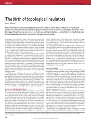
Static Column Expts (Well 1)Biocolloid Recovery vs Total Metal Content100.00%Cumulative Recovery (Log sum C/Co)10.00%1.00%0.10%Oocystsy = 213.1e -0.25xR 2 = 0.823-µmy = 12847e -0.30xR 2 = 0.690.01%30 35 40 45 50 55 60Total Metals (mg/g sediment)

Fundamentals of the scanning probe microscopyThe recently developed modes of restoration of the SPM images based on computer processing ofthe SPM data accounting the specific form of the tip allow only a partial solution of the problem[17,18]. The most effective mode of restoration is the numerical deconvolution [18], using the tipimage obtained experimentally by scanning test structures with a well-known topography. We shallillustrate the procedure with a one-dimensional example. If the tip shape is described by thefunction P(x), and the surface topography is described by the function R(x), then the SPM imageI(x) is given by the following relation:I (a) = R (x k ) - P (x k -a), under condition that dR/dx = dP/dx in x k points of contact.where a is the tip bias in surface coordinates. Partial restoration of the initial surface topography ismade by an inverse transformation: the SPM image is numerically scanned by an inverted tip. Thenthe restored topography image R′(x) is:R′(x) = I(x k1 ) - P(x - x k1 ), under condition that dI/dx = dP/dx in x k1 points of contact.Here x k1 is the abscissa of the point of contact of the SPM image function with the inverted tipfunction (i.e. with reversed directions for Y and X axes).It is necessary to note, that the full restoration of the sample surface would be possible only if thefollowing two conditions were satisfied: first, during scanning the tip has touched all points of thesurface, and, second, the tip has been always touching only one point of the surface. If the tipcannot reach some area of the surface during scanning (for example, if the sample has overhangingparts of topography), then only partial restoration of the topography can be performed. Inconclusion, the more points of the surface were touched by the tip during scanning, the morefaithfully it is possible to reconstruct the surface.32

Chapter 1. The scanning probe microscopy technique(а)(b)(c)(d)Fig. 35. Modeling of the surface topography restoration process(a) – initial surface with a relief shaped as a parallelepiped;(b) – modeling form of the tip as a paraboloid of revolution;(c) – result of convolution of the tip and initial surface;(d) – restored image of the surface.(Dimensions of images on X, Y, Z axes are specified in relative units).In practice the SPM image and the experimentally obtained tip shape are two-dimensional arrays ofdiscrete values for which the derivative is an ill-defined value. Therefore in practice instead ofderivation of discrete functions during numerical deconvolution of the SPM images, therequirement of minimality of the tip-surface distance is used during scanning with a constantaverage height [17]:Min {I(x k1 ) - P(x-x k1 )} .In this case it is possible to accept the minimal distance between the tip point and the correspondingpoint of a surface for the given position of the tip with respect to the surface as the topographicheight. This requirement in its physical sense is equivalent to the requirement of equality ofderivatives; however, it allows to search the points of a tip-surface contact with a more adequatemethod, which essentially reduces the time of topography reconstruction.33

Fundamentals of the scanning probe microscopySpecial test structures with known topography are used for calibration and determination of theform of the working part of the tip. Two SEM images of the most commonly used test structuresand their characteristic images, obtained by scanning-force microscope are shown in Fig. 36 andFig. 37.Fig. 36. Rectangular calibration lattice and its SFM imageFig. 37. Calibration lattice made of sharp pins and its SFM imageobtained by a pyramidal tip34

Chapter 1. The scanning probe microscopy techniqueThe calibration lattice made of sharp pins allows to image the tip apex while the rectangular latticehelps to restore the form of the tip lateral surface. Combining the results obtained by scanning theselattices, it is possible to restore completely the form of the working part of tips.Fig. 38. Electron microscope image of an SPM tipduring scanning of a test structure35

Fundamentals of the scanning probe microscopy2. Operating modes in scanning probe microscopy2.1. Scanning tunneling microscopyHistorically, the first microscope in the family of probe microscopes is the scanning tunnelingmicroscope. The working principle of STM is based on the phenomenon of electrons tunnelingthrough a narrow potential barrier between a metal tip and a conducting sample in an externalelectric field.E∆ZA 0ϕA tZFig. 39. Scheme of electrons tunneling through a potential barrier in STMThe STM tip approaches the sample surface to distances of several Angstroms. This forms a tunneltransparentbarrier, whose size is determined mainly by the values of the work function for electronemission from the tip ( ϕT) and from the sample ( ϕS). The barrier can be approximated by a*rectangular shape with effective height equal to the average work function ϕ :* 1ϕ = ϕ + ϕ ).2(T SFrom quantum mechanics theory [19,20], the probability of electron tunneling (transmissioncoefficient) through one-dimensional rectangular barrier is :WAt=2A02≅ e−k∆Z,Awhere0is the amplitude of electron wave function approaching the barrier;tthe amplitude ofthe transmitted electron wave function, k the attenuation coefficient of the wave function inside thepotential barrier; ∆ Z the barrier width. In the case of tunneling between two metals the attenuationcoefficient isA36

Chapter 2. Operating modes in scanning probe microscopyk*4π 2mϕ= ,hwheremis the electron mass,*ϕ the average electron emission work function, h the Planckconstant. If a potential difference V is applied to the tunnel contact, a tunneling current appears.E F1eVE F2Fig. 40. Energy level diagram of tunneling contact between two metalsBasically, electrons with energy near the Fermi level participate in the tunneling process.In case of contact of two metals the expression for the tunneling current density (in one-dimensionalapproximation) is [21,22]:jt****[ ϕ exp( −Aϕ ∆Z ) − ( ϕ + eV )exp( −A+ eV ∆Z )]= jϕ, (1)0E Fwhere the parametersj 0and A are set by the following expressions:j0e4π= , A = 2m.22 π h ( ∆Z)hFor small values of the bias voltage ( eV < ϕ ), the current density can be approximated by asimpler expression. The first order approximation in the series expansion of*exp( −Aϕ + eV ∆Z ) in expression (1) gives:jt=jexp( −A⎛⎛* ⎜ * *ϕ ∆Z ) ⋅ ϕ − ( ϕ + eV ) ⋅ ⎜1−⎜⎝⎝AeV∆Z⎞⎞⎟⎟*2 ϕ⎟⎠⎠0.*Finally, for eV

Fundamentals of the scanning probe microscopySince the exponential dependence is very strong, an even simpler formula is frequently used forestimations and qualitative reasoning:j t=4π− 2 mϕ*∆Zj (V )e h0, (2)in which the value j 0 (V ) is assumed to be not dependent on the tip-sample distance. For typicalvalues of the work function ( ϕ ~ 4 eV) the attenuation coefficient k is about 2 Å -1 so, when ∆ Zchanges of about 1 Å, the current value varies of one order of magnitude. Real tunneling contacts inSTM are not one-dimensional and have more complex geometry; however, the basic features oftunneling, namely the exponential dependence of the current on the tip-sample distance, are thesame also in more complex models, as proved by experimental results.ϕ*For large values of bias voltage ( eV > ), the well-known Fowler – Nordheim formula forelectron field emission into vacuum is derived from expression (1):J3 2e V=*8πhϕ( ∆Z )2⎡⎢ 8πexp −⎢⎣*2m(ϕ )3ehV32⎤∆Z⎥⎥⎦.The exponential dependence (2) of the tunneling current on distance allows adjusting the tip-sampledistance in a tunneling microscope with high accuracy. The STM is an electromechanical systemwith a negative feedback. The feedback system FS keeps the tunneling current value at the constantlevel (I 0 ), selected by the operator. The control of the tunnel current value, and consequently of thetip-sample distance, is performed by moving the tip along the Z axis with the help of a piezoelectricelement (Fig. 41).FSI 0IVFig. 41. Simplified block-diagram of the feedback in STM38

Chapter 2. Operating modes in scanning probe microscopyThe image of a surface topography in STM is formed in two ways. In the constant current mode(Fig. 42 (a)) the tip moves along the surface, performing raster scanning; during this the voltagesignal applied to the Z-electrode of a piezoelement in the feedback circuit (keeping constant the tipsampledistance with high accuracy) is recorded into the computer memory as a Z=f(x,y) function,and is later plotted by computer graphics.I t = constZ(a)XZ = constI t(b)XFig. 42. Formation of STM images in the constant current mode (a)and in the constant average distance mode (b)During investigation of atomic-smooth surfaces it is often more effective to acquire the STM imagein the constant height mode ( Z = const ). In this case the tip moves above the surface at a distanceof several Angstrom, and the tunneling current changes are recorded as STM image (Fig. 42 (b)).Scanning may be done either with the feedback system switched off (no topographic information isrecorded), or at a speed exceeding the feedback reaction speed (only smooth changes of the surfacetopography are recorded). This way implements very high scanning rate and fast STM imagesacquisition, allowing to observe the changes occurring on a surface practically in real time.The high spatial resolution of the STM is due to the exponential dependence of the tunnelingcurrent on the tip-sample distance. The resolution in the direction normal to the surface achievesfractions of Angstrom. The lateral resolution depends on the quality of the tip and is determined39

Fundamentals of the scanning probe microscopybasically not by the macroscopic radius of curvature of the tip apex, but by its atomic structure. Ifthe tip was correctly prepared, there is either a single projecting atom on its apex, or a small clusterof atoms, whose size is much smaller than the mean curvature radius of the tip apex. In fact, thetunneling current flows between atoms placed at the sample surface and atoms of the tip. The atom,protruding from the tip, approaches the surface to a distance comparable to the crystal latticespacing. Since the dependence of the tunneling current on the distance is exponential, the currentbasically flows in this case between the sample surface and the projecting atom on the apex of thetip.Fig. 43. Atomic resolution in a scanning tunneling microscopeUsing such tips it is possible to achieve a spatial resolution down to atomic scale, as demonstratedby many research groups using samples from various materials.Tips for tunneling microscopesTips of several types are used in scanning tunneling microscopes. In the beginning tips made from atungsten wire by electrochemical etching were widely used. This technology was well known andwas used for field-emission microscopes. The preparation of STM tips using this technology is thefollowing. A tungsten wire segment is fixed so that one of its ends passes through a conductingdiaphragm (D) that keeps a drop of alkali KOH in water solution (Fig. 44)40

Chapter 2. Operating modes in scanning probe microscopyWDKOHFig. 44. Scheme of a device for tungsten wire electrochemical etching to prepare STM tipsFeeding an electric current through the wire and the KOH solution, tungsten etching occurs. As faras etching goes, the thickness of the etched area gets smaller until the wire breaks, due to weight ofits bottom part. The bottom part falls down, automatically switching off the electric circuit andterminating the etching.Another widely used technique of STM tips preparation is cutting of a thin wire from Pt-Ir alloyusing ordinary scissors. The cutting is made at an angle about 45 degrees with simultaneous Ptension of the wire to tear it apart (Fig. 45).41

Fundamentals of the scanning probe microscopyPFig. 45. Schematic picture of the STM tip preparation by cutting a Pt-Ir alloy wireThe wire is cut while applying a stretching force P that produces a plastic deformation of the wire.As a result, in the place of cutting an extended apex with a ragged (curled) edge is formed withseveral protrusive defects, one of which becomes the working element of the STM tip. Thismanufacturing technique of STM tips is now used in all laboratories and provides almost always theguaranteed atomic resolution.Fig. 46. STM image of atomic structure of pyrolitic graphite42

Measurement of the local work function with STMChapter 2. Operating modes in scanning probe microscopyFor non-uniform samples the tunneling current is not only a function of tip-sample distance, butalso depends on the local value of the work function on the sample surface. The method of tipsampledistance modulation is used to obtain a map of the work function. For this purpose, duringscanning, a variable voltage with frequency ω is added to the control voltage of the scanner Z-electrode. The voltage applied to the Z-electrode of the scanner is thereforeU ( t ) = U + U sin( ω t )0 m.The tip-sample distance becomes modulated at the frequency ω:∆ Z ( t ) = ∆ Z + ∆ Z sin( ω t )0 m, where ∆ Z m and are related by the scannerpiezoelectric coefficient K:K = ∆ Z mU mThe value of the frequency ω is selected higher than the maximum frequency of the bandwidth ofthe feedback loop so that the feedback system cannot react to the tip-sample distance modulation.The amplitude of the voltage U m is small enough to be neglected in the weak dependence of thetunneling current on the applied voltage.U mU m·sin(ωt)~FSFig. 47. Setup for local work function measurementIn turn, the oscillations of the tip-sample distance modulate the current at the frequency ω :I t[ ∆Z+ ∆Z m sin( ωt)]*−αϕ≅ I (V )e020, where α = 2m.h43

Fundamentals of the scanning probe microscopySince the modulation amplitude is small, the tunneling current can be written asIt( ω t)≅Io( V)e−αϕ ∆ Z0[ 1 − α ϕ ∆ Z sin( ω t )]Thus, the amplitude of the small tunneling current oscillations with frequency ⎤ is proportional tothe square root of the local work function:2KUIω I02mh( x, y )m= ϕ *.Measuring the tunneling current amplitude oscillations in each point of the frame, it is possible tobuild a map of the local work function ϕ (x, y) simultaneously with the Z = f (x, y) topography onthe scanned area of a sample.m.Measurement of tunnel contact volt-ampere characteristicsUsing STM it is possible to measure the tunnel contact volt-ampere characteristics (VAC or I-Vcurves) that give information on the local conductivity of the sample and on the local density ofelectron states. The following procedure is the following. The sample area where measurementswill be performed, is selected on a previously acquired STM image. The STM tip is moved by thescanner to the first point of the selected area. To acquire I-V curves the feedback is broken for ashort time, and a linearly increasing voltage is applied to the tunneling junction. During the ramp,both the current flowing through the junction and the applied voltage are recorded.FSV=V (t)Fig. 48. Schematic picture of the tunneling junction I-V curves acquisitionSeveral I-V curves are measured in every point. Final volt-ampere characteristic is obtained byaveraging the I-V set, measured in one point. Averaging allows to minimize the influence of noise.44

Chapter 2. Operating modes in scanning probe microscopySTM control systemA simplified block diagram of the STM control system is presented in Fig. 49. The STM controlsystem consists of a digital part implemented by a personal computer, and an analog part, providedusually as a standalone block. The digital part consists of DAC and ADC sets and is enclosed on thescheme by red dotted border. The analog part is enclosed by a blue dashed line. The voltage Uapplied to the tunnel junction is set by the operator through a DAC, and the current I, controlled bythe feedback system, is also set through a DAC. Two-channel digital-to-analog converters (DAC-Xand DAC-Y) provide horizontal and vertical raster-scanning. The feedback loop is made of thepreamplifier PA (located in the STM measuring head), the differential amplifier DA, the lowfrequencyfilter LFF, amplifiers A4 and A5, and the piezo-scanner, controlling the tunneling gap.A1DAC - XA2DAC - YDAC - UDAC - IPAADCPFSDDALFFDAC - DGPSSKA4A3A5Fig. 49. The block diagram of an STM control systemThe operator first select suitable values for the working parameters (tunneling current and appliedvoltage) then starts the procedure for the tip-sample approach, by feeding a control voltage to themotor through the DAC–D converter. In the initial state there is no current in the feedback loop, andthe scanner is extended as much as possible toward the sample. When the tunneling current appears,45

Fundamentals of the scanning probe microscopythe feedback start retracting the scanner, while the system switches to a feedback mode. In thismode while the scanner is retracting the step motor approaches the sample to the tip until thescanner sets in the middle of its dynamic range. The value of a tunneling current set by the operatoris kept constant in the feedback loop during the approach.The sample scanning is performed by feeding a saw tooth voltage to external electrodes of thetubular scanner through the DAC–X and DAC–Y and the high-voltage amplifiers A1 and A2.During scanning the feedback system keeps the tunneling current constant. The real instantaneousvalue of the tunneling current I t is compared by the differential amplifier to the value I 0 , preset bythe operator. The differential signal (I t – I 0 ) is amplified (by A4 and A5 amplifiers) and fed to theinner Z-electrode of the scanner. Thus, the voltage applied to the Z-electrode during scanningreproduces the surface topography. The signal from the A4 amplifier output is digitized by the ADCconverter and stored in the computer memory.To acquire the information on the local work function distribution the signal produced by thegenerator G is added by the amplifier A5 to the Z-electrode voltage. The signal corresponding to thetunneling current modulation at frequency ω is selected by band-pass filter (PF) and measured bythe synchronous detector SD, driven by the reference voltage supplied by the signal generator G.The phase of the reference voltage is controlled by the phase shifter PS. The amplitude of thecurrent modulation is recorded in the computer memory as a signal proportional to the local workfunction.The measurement of the tunneling junction I-V curves in a set point of a sample is performed asfollows. The feedback is switched off for a short time using the electronic switch K. The voltage onthe inner electrode of the piezo-tube is kept constant by the capacitor C so that the tip hangs abovethe surface for a short time. After that the saw tooth voltage U (t) is applied to the tunnelingjunction from the converter DAC – U, and synchronously with it the tunneling current from thepreamplifier PU output is recorded in ADC. After that the switch K is closed, and the feedbacksystem restores the tunneling contact state corresponding to the I t = const condition. If necessary,the measurement of I-V curves is repeated N times to calculate an average curve.Scanning tunnel microscope designToday hundreds of different scanning probe microscope designs are described in the literature. Onone hand, such variety SPMs is caused by practical necessity, since certain SPM configuration isneeded to solve specific tasks. On the other hand, the relative simplicity of some SPM mechanicalpart stimulates manufacturing of measurement heads customized for specific experiments designedin research laboratories.The structure of STM measuring head must satisfy a lot of requirements in order to achieve asatisfactory performance. The most important requirement is high noise immunity. It is due to thehigh sensitivity of the tunneling gap to external vibrations, to temperature drifts, to electric andacoustic interference. Wide experience has been accumulated during last decade in this direction;many ways of shielding STM from influence of external factors have been developed. Finally, thechoice of the vibration isolation and thermal compensation system is dictated, basically, by theconvenience of use.As an example, an STM head design, with thermal drift compensation of the tip position, isschematically shown on Fig. 50.46

Chapter 2. Operating modes in scanning probe microscopy125634Fig. 50. An example of STM measuring head design1 - base; 2 – tubular three-coordinate piezo-scanner;3 – temperature-compensating piezo-tube, serving as a working elementof a step-by-step piezo-motor; 4 –tip; 5 – sample;6 - cylindrical sample holderThe base (1) holds two coaxial piezoceramic tubes of different diameter. The internal tube (2) playsthe role of a three-axes piezo-scanner. The external tube (3) performs a double task. First, theexternal tube cancels the deformations due to temperature changes, stabilizing the tip position in thedirection normal to the sample surface. Second, it is the working element of a step-by-step piezomotor,serving to approach the tip to the sample. The whole STM construction has axial symmetrythat reduces tip position thermal drift in the plane of the sample surface.Tunneling spectroscopyThe scanning tunnel microscope allows to record volt-ampere characteristics (VAC) of tip-surfacetunneling contact in any point of a surface and to investigate the local electric properties of asample. With the typical values of about 0.1–1 V for the bias of the tunneling contact and tunnelingcurrents at a level of 0.1÷1 nA, the order of magnitude of the tunneling contact resistance R t is10 8 ÷10 10 Ohm. As a rule, the R S resistance of samples studied in STM is much less than R t and theVAC is defined, basically, by the properties of a small sample area near the tunneling contact.47

Fundamentals of the scanning probe microscopyR SR S

Chapter 2. Operating modes in scanning probe microscopyIn this case the dependence of the tunneling current on the voltage is determined, basically, by thedensity of states in the sample. In practice the ρS( E ) value is estimated from the value of thetunneling current derivative with respect to voltage:∂ Iρ ( eV ) ≈ .S∂ VMeasurements of local tunneling spectra of various materials is performed, as a rule, in highvacuum (since the tunneling current is very sensitive to the state of the sample surface) and at lowtemperatures (since the thermal excitations strongly dither the features in the collected spectra).Metal - metal tunneling junctionElectron tunneling through a barrier between two metals was studied in many experimental workslong before the STM invention [27,28]. As it has been shown above, for small bias voltages thedependence of the tunneling current on the bias voltage is linear, and the conductivity of thetunneling contact is defined, basically, by the barrier shape:j t=4π−j (V ) e h2mϕ*∆Z0.At very high voltages the barrier shape will strongly change, and the current will be described bythe Fowler-Nordheim formula. A typical VAC, observed for metal-metal tunneling contacts, isrepresented schematically on Fig. 53.IVFig. 53. Generic metal-metal tunneling contact VACAs it can be seen from the figure, the volt-ampere characteristic of the metal-metal tunnelingcontact is nonlinear and, as a rule, it is practically symmetric.49

Fundamentals of the scanning probe microscopyMetal–semiconductor contact VACSemiconductor samples have more complex structure of the electron energy spectrum.IE FPE gE FSVFig. 54. Energy levels and generic VAC for metal-semiconductor tunneling contactPresence of an energy band gap and impurity levels in semiconductor materials makes the VAC ofa metal-semiconductor tunneling contact strongly nonlinear. Essential contribution to the tunnelingcurrent is made also by the surface states and by the energy levels due to foreign atoms adsorbed onthe surface. Therefore measurements of local tunneling spectra of semiconductor materials areperformed in high vacuum. Uncontrollable presence of adsorbed atoms on the surface stronglycomplicates the interpretation of the tunneling spectra obtained in experiment. Besides that, thermalexcitations result in significant widening of discrete energy levels corresponding to localized states,and also strongly dither the position of the conduction and valence band edges. As an example, thetunneling spectrum of a GaAs sample [29] is presented on Fig. 55.(dI/dV) / (I/V)6E VE C420-2 - 1 0 1 2VFig. 55. STM spectrum of a n-GaAs crystal surfaceTunneling spectra allow to determine the position of the edges of the conduction and valence bandwith respect to the Fermi level, and also to identify the spectral peaks due to impurity states insidethe energy gap in semiconductors.50

Chapter 2. Operating modes in scanning probe microscopyBaseCantileverTipFig. 59. AFM probe schematic pictureThe interactive forces measured by AFM can be qualitatively explained by considering, forexample, the van der Waals forces [32]. The van der Waals potential energy of two atoms, locatedat a distance r from each other, is approximated by the exponential function - Lennard-Jonespotential:612⎧ ⎛ r⎫0 ⎞ ⎛ r0⎞U LD( r ) = U ⎨−2⎜⎟ +0 ⎜ ⎟ ⎬ .⎩ ⎝ r ⎠ ⎝ r ⎠ ⎭The first term of the sum describes the long-distance attraction caused, basically, by a dipole-dipoleinteraction and the second term takes into account the short range repulsion due to the Pauliexclusion principle. The parameter r 0 is the equilibrium distance between atoms, the energy valuein the minimum.U LDr orU 0Fig. 60. Lennard-Jones potential qualitative formLennard-Jones potential allows to estimate the interaction force of a tip with a sample [33]. Theenergy of the tip-sample system can be derived, adding elementary interactions for all the tip andsample atoms.53

Fundamentals of the scanning probe microscopyr 'r-r 'rFig. 61. How to calculate the energy of interaction between tip and sample atomsThen for the energy of interaction we get:W PS = ∫∫U LD (r − r ′) n P ( r ′)n S (r) dV d V ′ ,V P V Swhere n S (r) and n P ( r ′) are the densities of atoms in the sample and in the tip. Accordingly, theforce affecting the tip from a surface can be calculated as follows:rF = −grad(W).PSPSGenerally this force has both a component normal to the sample surface and a lateral component(laying in the plane of the sample surface). Actual interaction of a tip with a sample has morecomplex character; however, the basic features are the same : the AFM tip is attracted by the sampleat large distances and repelled at small distances.Acquisition of an AFM surface topography may be done by recording the small deflections of theelastic cantilever. For this purpose optical methods (Fig. 62) are widely used in atomic forcemicroscopy (the technique named beam-bounce).LaserPhoto diodePhoto diode(1)(2)(3)(4)Fig. 62. Schematic description of the optical system to detect the cantilever bending54

Chapter 2. Operating modes in scanning probe microscopyThe optical system is aligned so that the beam emitted by a diode-laser is focused on the cantilever,and the reflected beam hits the center of a photodetector. Four-section split photodiodes are used asposition-sensitive photodetectors.(1)(2)(1)(2)(3)(3)(4)(4)F Z(a)F L(b)Fig. 63. Relation between the types of the cantilever bending deformations (bottom)and the change of the spot position on the split photodiode (top)Two quantities may be measured by the optical system: the cantilever bending due to attractive orrepulsive forces (F Z ) and the cantilever torsion due to lateral components (F L ) of the tip-surfaceinteraction forces. If reference values of the photocurrent in the photodiode sections are designatedas I 01 , I 02 , I 03 , I 04 , and I 1 , I 2 , I 3 , I 4 are the current values after change of the cantilever position,then differential currents from various sections of the photodiode ∆I i = I i - I 0i will characterize thevalue and the direction of the cantilever bending or torsion. In fact, the following current difference∆ I z = (∆ I 1 +∆I 2 )−(∆ I 3 +∆I 4 )is proportional to the cantilever bending due to a force normal to the sample surface (Fig. 63 (a)),and the following combination of differential currents∆ I L =(∆ I 1 +∆I 4 )−(∆ I 2 +∆I 3 )characterizes the cantilever bending due to lateral forces (Fig. 63 (b)).The ∆I Z value is used as an input parameter in a feedback loop of the atomic force microscope(Fig. 64). The feedback system (FS) keeps ∆I Z = const with the help of a piezoelectric transducer(scanner), which controls the tip-sample distance in order to make the bending ∆Z equal to thevalue ∆Z 0 preset by the operator.55

Fundamentals of the scanning probe microscopy∆I zPhotodiodeLaserDiodeFS∆I Z0FSZPiezoactuatorFig. 64. Simplified scheme of the feedback in an optical lever detection AFMWhen scanning a sample in a ∆Z = const mode the tip moves along the surface, thus the voltage onthe scanner Z-electrode is recorded in the computer memory as a surface topography Z = f (x, y).The AFM lateral resolution is defined by the radius of curvature of the tip and by the sensitivity ofthe system in detecting the cantilever deviations. Currently the AFM are designed to allowobtaining atomic resolution.AFM probesSurface sensing in the atomic force microscope is performed using special probes made of an elasticcantilever with a sharp tip on the end (Fig. 65). Such probes are produced by photolithography andetching of silicon, SiO 2 or Si 3 N 4 layers deposited onto a silicon wafer.Si∆ZFig. 65. Schematic picture of the AFM probe56

Chapter 2. Operating modes in scanning probe microscopyOne end of the cantilever is firmly fixed on the silicon base - the holder, and the tip is located on thefree cantilever end. The curvature radius of AFM tip apex is of the order of 1 ÷ 50 nanometersdepending on the type and on the technology of manufacturing. The angle near the tip apex is 10 ÷20º. The interaction force F of a tip with the surface can be estimated from the Hooke law:F= k ⋅ ∆Z,where k is the cantilever elastic constant; ∆Z is the tip displacement corresponding to the bendingproduced by the interaction with the surface. The k values vary in the range 10 -3 ÷ 10 N/mdepending on the cantilever material and geometry. The cantilever resonant frequency is importantduring AFM operation in oscillating modes. Self frequencies of cantilever oscillations aredetermined by the following formula (see, for example, [34]):λiEJ= , (3)l ρ Sωri 2where l is the cantilever length; E the Young’s modulus; J the inertia moment of the cantilevercross-section; ρ the material density; S the cross section; λ ia numerical coefficient (inthe range 1÷100), depending on the oscillations mode.λ = 3 52λ = 22 04λ = 6171,2,3,Fig. 66. Main cantilever oscillations modesFrequencies of the main modes are usually in the 10÷1000 kHz range. The quality factor Q ofcantilevers mainly depends on the media in which they operate. Typical values of Q in vacuum are10 3 – 10 4 . In air the quality factor drops to 300 – 500, and in a liquid it falls down to 10 – 100.Basically, two types of probes are used in AFM –cantilever shaped as a beam of rectangular sectionand triangular cantilever, formed by two beams. A schematic picture of rectangular cantilever ispresented in Fig. 67.57

Fundamentals of the scanning probe microscopyFig. 67. A cantilever with rectangular sectionElectron microscope images of commercial cantilevers with rectangular cross section (NSG - 11probes produced by NT-MDT Company) are shown in Fig. 68.Fig. 68. SEM images of AFM tips on rectangular cantilevers [54]Sometimes the AFM probes have few cantilevers of various length (hence, of various stiffness aswell) on one base. In this case the working cantilever is selected by corresponding alignment of theAFM optical system.58

Chapter 2. Operating modes in scanning probe microscopyProbes with triangular cantilever have higher stiffness and, hence, higher resonant frequencies.They are usually used in oscillating AFM techniques. A schematic picture of triangular cantileversis shown in Fig. 69 and SEM images in Fig. 70.Fig. 69. Schematic picture of triangular cantileverFig. 70. SEM images of AFM tip on a triangular cantilever [54].Manufacturing of AFM probes is a complex technological process including photolithography, ionimplantation,chemical and plasma etching operations. The basic stages of one of possible probemanufacturing techniques are presented in Fig. 71.59

Fundamentals of the scanning probe microscopyThe AFM probe manufacturing techniques1Si (110)82Photoresist394Si 3 N 45106711Fig. 71. Basic stages of the probe manufacturing process60

Chapter 2. Operating modes in scanning probe microscopyWafer of single crystal silicon (110) are used for probe manufacturing. A thin photoresist layer(Fig. 71, stage 2) is deposited on the wafer surface. Then photoresist is exposed through a photomask, and a part of photoresist is removed by means of chemical etching. After that ions of boronare implanted to a depth of about 10 microns into the silicon area, unprotected by photoresist (stage3). The photoresist is further washed off in a special etching agent, and then the wafer is thermallyannealed, resulting in atoms of boron diffusing into the silicon crystal lattice. The silicon alloyed byboron, forms a so-called stop-layer which blocks the process of etching for some selective etchingagents. Then on the reverse side of the wafer the photolithography is done again, as a result ofwhich the photoresist layer is formed exactly above the area implanted by boron. After that thewafer is covered by a thin Si 3 N 4 layer (stage 4). Then the photoresist is selectively etched, andduring dissolution photoresist bloats and strips off the thin Si 3 N 4 film located directly above it(stage 5). The silicon plate is etched through to the stop-layer by the selective etching agent, whichreacts with silicon and does not react with alloyed silicon and Si 3 N 4 layer, (stage 6). After that Si 3 N 4is washed off, and photoresist islands are formed on the reverse side of the wafer in the alloyed areaby a photolithography method (stages 7,8). Then the silicon is etched, resulting in formation ofcolumns of silicon under photoresist islands (stage 9). After that needles are formed with the help ofplasma etching from silicon columns (stages 10,11). Cantilevers from the reverse side (with respectto the apex) are covered with a thin layer of metal (Al, Au) to improve the reflective properties. Asa result of these operations a set of hundreds probes is made on one silicon wafer. For electricmeasurements the conducting coatings from various materials (Au, Pt, Cr, W, Mo, Ti, W 2 C, etc.)are applied on a tip. Tips in magnetic AFM probes are covered with thin layers of ferromagneticmaterials, such as Co, Fe, CoCr, FeCr, CoPt, etc.The contact mode in atomic force microscopyThe methods used in AFM to acquire images (either topographic or related to local sampleproperties) can be split in two groups : the contact modes (quasi-static) and the non-contact modes(oscillatory).In contact mode the tip apex is in direct contact with the surface, and the force (attractive orrepulsive) acting between the atoms of tip and sample is counterbalanced by the elastic forceproduced by the deflected cantilever. Cantilevers used in contact-mode have relatively smallstiffness, allowing to provide high sensitivity and to avoid undesirable excessive influence of the tipon the sample.The contact mode may be carried out either at constant force or at constant average distance(between probe and sample). During scanning in constant force mode the feedback system providesa constant value of the cantilever bend, and consequently, of the interaction force as well (Fig. 72).Thus the control voltage in the feedback loop, applied to the Z-electrode of the scanner, will beproportional to the sample surface topography.Scanning at constant average distance between the tip and the sample (Z = const) is frequently usedon samples with small roughness (a few Angstrom). In this mode (also named constant heightmode) the probe moves at some average height Z av above the sample (Fig. 73) and the cantileverbend ∆Z, proportional to the applied force, is recorded in every point. The AFM image in this casedescribes the spatial distribution of the interaction force.61

Fundamentals of the scanning probe microscopyF z = constZZScanningXFig. 72. AFM image acquisition at constant force∆ZZ av = const∆Z, F zXScanningFig. 73. AFM image acquisition at constant average distance (constant height)A drawback of contact modes is the direct mechanical interaction of the tip with the sample. Itfrequently results in tips breakage and/or sample surface damages. Contact techniques arepractically not suitable for soft samples such as organic and biological materials.Dependence of the force on the probe-sample distanceWith the help of the atomic force microscope it is possible to study detailed features of the localforce interaction, yielding information on the sample surface properties. With this purpose the socalledforce-distance curves (tip approaching to, or retracting from the surface) are measured.Actually these are the dependences of the cantilever bending ∆ Z (and consequently, of theinteraction force) on the coordinate z, i.e on the probe-sample distance. A typical ∆ Z = f ( z )curve is shown in Fig. 74.62

Chapter 2. Operating modes in scanning probe microscopy∆Z, Fz(a)z(b)Fig. 74. Schematic picture of the cantilever deflection ∆Z (proportional to the applied force F)versus the probe-sample distance z. Blue: approaching. Red: retractingDuring approach to the surface the tip gets in the reach of attractive forces. This causes a cantileverbend toward the surface (Fig. 74, insert (a)). The jump of the tip to the surface is due to the largegradient of the attractive force near the sample surface. For a Lennard-Jones type potential the range'Z* of the attractive force, where the gradient F zis high, is about 1 nanometer. The behavior of theLennard-Jones force and its derivative with respect to the tip-surface distance is schematicallyshown in Fig. 75.FF´zZ*zZ*zr o(a)r o(b)Fig. 75. Schematic picture of the force (a) and of the force gradient (b)as functions of the tip-surface distance z.The jump of the tip to the surface may be observed only when the cantilever elastic constant issmaller than the maximum force gradient. This can be explained by considering the motionequation of an elastic cantilever near the surface:mz&1= −kz1+ F( d + z1)& ,where d is the tip-surface distance at equilibrium andthe displacement from the equilibriumposition, F(z) the tip-surface interaction force, k and m are the cantilever elastic constant and mass.z 163

Fundamentals of the scanning probe microscopyUsing a linear approximation of the function F(z) we get:F = F( d ) + F ′z( d ) ⋅z 1[ k − F ′(d )] z F ( d )m z ′ +=z′ .1 1With the substitution,2z′ + ω z 0 ,2 0 2=F( d )z 2= z 1−k − , the motion equation takes the form:F ( d )z ′k − F ′2 ( d )zω0=.mIn this form it becomes apparent that the oscillator frequency ω0depends on the distance d. If the2force gradient at any distance is larger than the cantilever elastic constant, then ω0< 0 . Thiscondition corresponds to the unstable equilibrium position of an inverted pendulum. Any smalldisturbance results in loss of stability, and the cantilever moves to the surface.During further approach of the probe to the sample, the tip starts to experience a repulsive force,and the cantilever bends in the opposite direction (Fig. 74, insert (b)). The slope of the curve∆Z = f (z) in this region is determined by the elastic properties of both sample and cantilever. Ifinteraction is perfectly elastic, the dependence of the bend on the distance, recorded during reversemotion, coincides with the dependence obtained during forward motion (Fig. 74). For soft (plastic)samples, such as films of organic materials, biological structures, etc., and also for samples withadsorbed layers of various materials, the shape of the ∆Z = f (z) curves is more complex. In thiscase the shape of the curve is strongly influenced by the capillary and plasticity effects. As anexample, approach-retraction curves for a sample coated by a layer of a liquid are schematicallyshown in Fig. 76, where the hysteresis due to capillary effect is apparent. During probe approach tothe sample the tip is wetted by the liquid (at the ″snap-on″ distance z 1 ), and a meniscus is formed.The tip, submerged in the liquid, is affected by an additional force of surface tension. Duringretraction the tip-liquid separation occurs at a larger distance (″snap-off″ distance z 2 > z 1 ).∆Z, Fz 1 z 2zFig. 76. Schematic picture of the cantilever deflection ∆Z (proportional to the applied force F)versus the probe-sample distance z , on a sample with an adsorbed liquid layer64

Chapter 2. Operating modes in scanning probe microscopyThus, by the shape of the ∆Z = f (z) curve it is possible to obtain information on the tip-surfaceinteraction, to study the local stiffness of the sample and the distribution of the adhesion forces.AFM control system in the contact modeThe simplified circuit of the AFM control system during cantilever operation in the contact mode ispresented in Fig. 77. The control system consists of a digital part implemented by a personalcomputer, and an analog part, usually a stand-alone block. The digital part contains, basically,digital-to-analog (DAC) and analog-to-digital (ADC) converters. Two-channel digital-to-analogconverters DAC-X and DAC-Y provide the sample raster-scanning. The feedback loop consists ofthe preamplifier PA structurally located in the AFM measuring head, a differential amplifier (DA),high-voltage amplifier A2 and a piezo-transducer, regulating the bend value of a cantilever, andconsequently, the tip-surface interaction force. In the initial state the analog switch SW 1 is closed,and SW2 is open.PhotodiodePALaserSW2DAC - UA1DAC - SetADC"Z"UDAU 0A3DAC - SMSMA4DAC - XSW1A5DAC - YA2DAC - ZFig. 77. Simplified circuit of the control system during operation in the contact mode65

Fundamentals of the scanning probe microscopyAt first the operator aligns the optical system, focusing the laser spot onto the cantilever andmaximizing the photodiode total current, while minimizing the difference between the oppositephotodiode sectors. Then, a voltage U 0 , proportional to the working value of the cantileverdeflection ∆Z (which will be kept constant by the feedback system) is established by means of theDAC-Set. After that the procedure for tip-sample approach is switched on: a control voltage fromDAC-SM is supplied to the stepping motor (SM). In the initial state the voltage in the feedback loop(proportional to the difference of currents between the photodiode vertical sectors) is smaller thanthe value established by the DAC-Set, and the scanner is extended as much as possible in thedirection of the tip. During approach the cantilever is bent, the differential photodiode currentincreases, and the system of approach passes to the procedure for optimizing the scanner dynamicrange. There is a further movement of the sample toward the tip provided by the stepping motor anda simultaneous retracting of the sample provided by the scanner (while the feedback keeps thecantilever bend constant) until the sample surface plane sets in the position corresponding to themiddle of the dynamic range of the scanner. After that the microscope is ready for operation.Scanning of a sample is performed by feeding a saw tooth voltage to the external electrodes of thetubular scanner through two-channel DAC-X and DAC-Y converters and two-channel high-voltageA4, A5 amplifiers. During the sample scanning, the value of the photodiode differential currentselected by the operator (corresponding to a certain value of the cantilever bend) is kept constant. Inthe constant force mode (F z = const) the voltage fed to the Z-electrode of the scanner isproportional to the surface topography. This happens as follows. The real time value of the voltageU, proportional to the differential photodiode current, is compared by the differential amplifier(DA) with the value U 0 , set by the operator. The differential voltage (also named “error signal”,∆U=U-U 0 ) is amplified (by A2) and supplied to the internal Z-electrode of the scanner. The scannerextends or retracts (with respect to the actual position set by the DAC-Z), depending on the sign ofthe signal ∆U, until ∆U becomes (practically) zero. Thus, during scanning the voltage applied to theZ-electrode of the scanner is proportional to the z-shift executed by the scanner in order to keepconstant the tip-surface distance, i.e. to the surface modulation in the z-direction . The output signalof the differential amplifier is recorded by ADC as information on the surface topography.It is possible to measure, in a selected point of the sample, the dependence of the cantileverdeflection on the probe-surface distance: ∆Z = f ( z). For this purpose the feedback is interrupted bythe analog switch SW1, and a saw tooth voltage is applied to the Z-electrode of the scanner fromthe DAC-Z. Synchronously the ADC records the output voltage of the preamplifier PA, which isproportional to the cantilever deflection and consequently, to the tip-surface interaction force. Theacquired data are transformed into a ∆Z = f ( z) curve, which can be plotted on the computerdisplay.Acquisition of the AFM image in the constant average distance mode (also named constant heightmode ) is done in the following way. In the beginning the ∆Z = f ( z) dependence is measured and a(small) distance of the tip above the surface is chosen. Then the feedback is broken, and the sampleis scanned. The preamplifier output voltage, proportional to the cantilever deflection, is recorded asinformation of the force distribution F(x,y) along the sample surface. For samples with smallroughness the ″constant height″ image gives information similar to the ″constant force″ image.Registration of volt-ampere characteristics of a tunneling tip-sample contact in a selected point of asurface is possible using cantilevers with a conducting coating. The SW2 switch is closed to obtainthe VAC, and a saw tooth voltage from the DAC-U is applied to the cantilever. Synchronously thevoltage, proportional to the current through the contact, is amplified (by A1), recorded by the ADCin the computer memory and plotted on the computer display.66

Chapter 2. Operating modes in scanning probe microscopyThe drawback of AFM contact techniques is the direct mechanical interaction of the tip with thesurface. It frequently results in breakage of tips and damage of the samples surface. Contacttechniques are therefore not appropriate for analysis of soft samples (organic materials or biologicalobjects). Soft samples are more successfully studied using an oscillating cantilever. Oscillatorytechniques strongly reduce the mechanical influence of the tip on the surface during scanning.Besides that, development of oscillatory techniques has essentially expanded the variety of surfaceproperties that can be investigated with AFM.Forced oscillations of a cantileverThe exact description of the AFM cantilever oscillations is a complex mathematical task. However,the basic features of the processes occurring during interaction of an oscillating cantilever with asurface can be understood on the basis of elementary models, in particular, using the approximationof a localized mass model [3]. Let us approximate the cantilever as an elastic massless beam (withelastic constant k), fixed at one end on the piezo-vibrator PV, plus a mass m localized on the otherend (Fig. 78).kz (t)mPVu=u (t)Fig. 78. Probe model as an elastic cantilever with a mass at one endLet the piezo-vibrator oscillate with frequency ω:u = u cos( ωt).0Then the motion equation of the system is,m & z= −k(z − u ) − γ z&+ , (4)F 0where the term γ z& , proportional to the first derivative, takes into account the viscous force in air,F 0and takes into account the gravity force and other possible constant forces. A constant forceonly displaces the equilibrium position of the system and does not influence the frequency, theamplitude and the phase of the oscillation. Therefore, with the variable substitution:z1+0= z F / k ,the motion equation for the displacement z 1 from the equilibrium position takes the form:m& z+ z&+ kz ku cos( ωt) .1γ1 1=0With the definition ω = k / m , and introducing the quality factor of the system Q = ω m / γ ,00we obtain:67

Fundamentals of the scanning probe microscopyω022& z+ z&+ ω z = ω u cos( ω t ) . (5)1 1 0 1 0 0QThe simplest solution is found in the domain of complex numbers η , by writing the equation in theform:ωQ0 22 −iωt& & η + ω η = ω u e .η+00 0where i is the imaginary unit.The general solution is the superposition of dumped oscillations with decrementδ = ω 0/ 2Qandpersistent forced oscillations with frequency ω. Let us find the steady-state oscillations. We searchfor a solution in the formη−iωt= a ⋅ e .Substituting (5) in the equation (4), we obtain for the complex amplitude a:2ω0u0a = .2 2 ωω0ω − ω − i0QThe module of a is the forced oscillations amplitude A(ω):A( ω )u ω20 0= . (6)2 22 2 2 ω ω0( ω0− ω ) +2QThe phase of the complex amplitude a is the phase difference ϕ(ω) between the system oscillationand the forcing term u = uo cos( ωt) :⎡ ωω ⎤0ϕ ( ω ) = arctg⎢⎥ . (7)2 2⎣Q(ω0− ω )⎦From expression (6) it follows, that the tip oscillation amplitude A(ω 0 ) = Q u 0 , at the frequency ω 0 ,is proportional to the quality factor. Besides that, presence of dissipation ( γ ≠ 0 , i.e. Q ≠ ∞ ) inthe system results in a decrease of the resonant frequency of the cantilever oscillations. Indeed,68

Chapter 2. Operating modes in scanning probe microscopy2differentiating the radicand with respect to ω in expression (6) and equating the derivative to zero,we obtain for the resonant frequency ω rd :2 ⎛ ⎞=2 1ω ⎜ − ⎟rdω01 .2⎝ 2Q⎠The shift of the dissipative system resonant frequency is⎛ 1 ⎞ω = ω − ω = ⎜⎟− −0 rdω 1 10.⎝ 2Q⎠∆2Increasing dissipation, the amplitude-frequency characteristic of the system (response curve) isshifted to lower frequencies (Fig. 79).AπϕQ = ∞ωQ ≠ ∞ωω rdω oω oFig. 79. Change of the amplitude-frequency characteristicand phase response in a system with dissipation.Blue color shows characteristics of non-dissipative system.However, for typical values of quality factor of cantilevers in air, the resonant frequency shift due todissipation is small. Influence of the dissipation amounts, basically, to essential reduction of theoscillations amplitude and to broadening of the amplitude and phase response curves of the system(Fig. 79).Contactless mode of AFM cantilever oscillationsIn a contactless mode the cantilever forced oscillations amplitude is small: about 1 nanometer.During tip to surface approach, the cantilever is affected by an additional force F PS(z) due to vander Waals interaction with the sample. For small oscillations of the cantilever around the distancefrom the surface, the force may be approximated by the first (linear) term in the seriesexpansion:z 069

Fundamentals of the scanning probe microscopyFPS∂F= FPS+ ( z0) ⋅ z( t ) = FPS0∂z+ F′⋅ z( t )0 z.where F′zis the gradient of the tip-surface interaction force at the distance z0. Therefore anadditional term must be included into the motion equation (4).m& z−k(z − u ) − γ z&+ F + F + F z .= ′0 PS 0 zWith the variables substitution:z0+PS 0= z + ( F F )/ k , we come to the following equation:m& z+ z&+ ( k − F ′z) ⋅ z = ku cos( ωt) .γ0I.e. presence of a force gradient results in a change of effective stiffness of the system:k= k − .'effF zThe motion equation (5) for the "free cantilever" oscillation (i.e. the cantilever at a distance fromthe surface that makes ′ negligible) changes into:F zω ⎛ 2 F ′z ⎞2& z&+ 0 z&+ ⎜ω0− ⎟ ⋅ z ω0u0cos( ω t )Q ⎝ m ⎠=.Repeating the calculations carried out for the free cantilever, we get the amplitude-frequencycharacteristic for the cantilever in the force gradient F′:A( ω )2=0 0. (8)2 22 2 2 2( ω − ω − F′/ m) + ω ω / Q0u ωAnd, accordingly, the phase response:z0⎡ ωω( ) ⎥ ⎤0ϕ ( ω ) = arctan⎢. (9)2⎣ ω − − F′0ω0z/ m ⎦Thus, presence of a gradient in the tip-surface interaction force results in additional shift of theamplitude and phase response curves. The resonant frequency ω rf in presence of external force canbe written as2 2⎛ 1 F′⎞z 2 F′zωrf= ω0⎜1−− ⎟ = ωrd− .2⎝ 2Qk ⎠ mzHence, additional shift of the amplitude-frequency characteristic is equal to⎛ F′⎞z∆ω = ω −ω= ω ⎜⎟1 − 1−.rd rd rd⎝ mωrd ⎠70

Chapter 2. Operating modes in scanning probe microscopyAϕω rfω rdωω*ω oωFig. 80. Change of the amplitude-frequency characteristic and the phase responseof a cantilever under influence of a force gradient.From expression (9) it also follows, that the presence of a force gradient shifts the phase responsecurve so that the inflection point occurs at the frequency ω * :F '*zω = ω 01 −Andk⎛ ⎞⎜F '*z∆ω = ω − ω = ω ⎟1 − 1 −0 0.⎝ k ⎠Let the cantilever perform forced “free” oscillations far from a surface with frequency ω0, then thephase shift is π/2. During approach to the surface the phase (assuming F z ′ < k ) changes to⎡ k ⎤ QF′z( ) arctan −QF⎥ ≈ πϕ ω = ⎢.0⎣ ′ kz ⎦ 2Hence, the additional phase shift in presence of a force gradient [35] will be equal to:π QF= − ϕ(ω ) ≅2k∆0'zϕ .The phase shift is therefore proportional to the force gradient. This effect is used obtain the phasecontrast AFM image."Semi-contact" mode of the AFM cantilever oscillationsIn order to detect changes in the amplitude and in the phase of cantilever oscillations in non-contactmode high sensitivity and stability of the feedback is required. In practice the so-called "semicontactmode" (also named "intermittent-contact mode" or "tapping mode") is used morefrequently. In this technique the forced cantilever oscillations are excited near a resonancefrequency with an amplitude about 10–100 nanometers. The cantilever is approached to the surfaceso that in the lower semioscillation the tip get in contact with the sample surface (this correspondsto the repulsive region in the force-distance diagram (Fig. 81)).71

Fundamentals of the scanning probe microscopyFig. 81. Working point selection during "semi-contact" modeDuring scanning, the changes of amplitude and phase of cantilever oscillations are recorded. Thecantilever interaction with the surface in "semi-contact" mode consists in van der Waals forces plusthe elastic force which is added during contact. If z 0 is the distance covered by the tip from theequilibrium position until contact with the surface, and F PS( z( t )) is the combined force, then themotion equation of the cantilever is:2ω20& z+ 0 z&+ ω [ z( t ) z u cos( t )] ω F [ z( t )]0−0−0ω =,PSQkwhere the origin of z coordinate is at the surface. We shall notice, that the "semi-contact" mode isrealized only when the z 0 distance is smaller than the amplitude of cantilever oscillations:z0< Q u 0.The theory of "semi-contact" mode is much more complex than the theory of contactless mode,since in this case the equation describing cantilever movement is essentially non-linear. TheF PS( z( t )) force now cannot be approximated by the first terms of a series expansion for small zvalues. However the characteristic features of this mode are similar to the features of a contactlessmode - the amplitude and the phase of cantilever oscillations depend on the tip-surface interactionin the bottom part of cantilever oscillations. Since in the bottom part of oscillations the tip interactsmechanically with the surface, then in this mode the sample local stiffness has essential influenceon the amplitude and phase changes.The phase shift between the piezoelectric vibrator driving signal and the stationary cantileveroscillation can be estimated by considering the energy dissipation process during tip-sampleinteraction [36-38]. In stationary oscillations the energy entering the system is exactly equal to the72

Chapter 2. Operating modes in scanning probe microscopyenergy dissipated by the system. The energyperiod is equal to:E EXsupplied by piezo-vibrator during one oscillationEEX=t+2π/ ω∫tdzku cos( ωt) ⋅ dtdt0 .This energy is spent compensate the losses due to interaction of the cantilever with the atmosphereand with the sample. The energy , dissipated in the atmosphere during one period, is:EPA=t+2π/ ω∫tω0⎛⎜Q ⎝mdzdt2⎞⎟⎠dt.E PATheE PSenergy spent to compensate the losses during dissipative tip-sample interaction, is:EPS=t+2π / ω∫tFPS(dzz )dtdt.From the equilibrium condition it follows that:E E + EEX= .PAPSAssuming stationary oscillations z = A ⋅ cos( ω t + ϕ ), we get:EPS2π ku A π kωA0= EEX− EPA= sin( ϕ ) − .Qω Q0Therefore, the phase shift can be obtained from the following equation:ω A QEsinϕ +ω 0u π kuPS= .00AThus, the cantilever oscillations phase shift in "semi-contact mode" is determined by the amount ofdissipative tip-sample interaction.Formation of the AFM image in "semi-contact mode" is done as follows. The piezo-vibrator drivesthe cantilever oscillations at frequency ω (close to a resonant frequency) and with amplitude A ω .During scanning the AFM feedback system keeps the oscillations amplitude constant at the A 0level, set by the operator (A 0 < A ω ). The voltage in the feedback loop (fed to the Z-electrode of thescanner) is recorded in the computer memory as topographic AFM image of the sample.Simultaneously, the change of the cantilever oscillation phase is also recorded as "phase contrastimage". As an example, the topographic and the "phase contrast" AFM images of a polythene film,obtained in "semi-contact" mode [54] are presented in Fig. 82.73

Fundamentals of the scanning probe microscopy(a)(b)Fig. 82. AFM images of a polythene film area surface, obtained in a "semi-contact" ("tapping") mode(a) - surface topography obtained in constant amplitude mode;(b) - corresponding distribution of phase contrast2.3. Electric force microscopyIn EFM the electric tip-sample interaction is used to collect information on the sample properties.Let us consider a system consisting of a probe, made of cantilever and tip with conducting coating,and a sample made of a thin layer of a material on a well conducting substrate.Conductingcoatingϕ (x,y )U ∼U 0Fig. 83. Measurement circuit of the electric tip-sample interactionLet the constant voltage U 0 and the variable voltage U ∼ = U 1·sin (ω t) be applied between the tipand the sample. If the thin layer on the substrate is a semiconductor or a dielectric the surfacecharge produces a potential distribution ϕ (x,y) on the sample surface. The voltage between the tipand the sample surface is:U= U0+ U1⋅ sin( ωt)− ϕ(x, y )74

Chapter 2. Operating modes in scanning probe microscopyand the tip-sample capacity C, under the bias voltage U, stores the energy:2CUE = .2Then electric force of tip-sample interaction isr.F = −grad(E )And the Z-component of the electric force acting on the tip isFz∂ E 1 2 ∂ C 12 ∂ C= − = − U = − [ U (x, y) U sin( ω t) ]0− ϕ +.1∂ z 2 ∂ z 2∂ z2that, remembering the identity sin ( t ) [ 1 cos( 2 t )] / 2ω= − ω , can be written:Fz1 ⎧1= − ⎨ 001122 ⎩222[ U − ϕ(x,y) ] + 2[ U − ϕ(x,y) ] U sin(ωt) + U [ 1 − cos( ωt) ]⎫ ∂ C⎬⎭ ∂ zFrom the last expression it follows, that the interaction force is the sum of three components:Fz( = 0 )⎧1⎛= −⎨⎜(U⎩2⎝0−ϕ(x, y ))21+ U221⎞⎫∂C⎟⎬⎠⎭∂zωconstant component;C{( U − ϕ(x, y ))⋅Usin( t )} zF z()−ω 1= ω∂∂0component at frequency ω ;⎧1 2 ⎫∂C= ⎨ U cos( ωt)1 ⎬⎩4⎭ ∂zF 2z( ω )component at frequency22 ω .A synchronous detection of the cantilever oscillation amplitude at frequency 2 ω allows to map, onthe sample surface, the quantity C ' z(x,y ), i.e. the derivative of the capacity with respect to the z-coordinate. This technique is named Scanning Capacitance Microscopy (SCM) [39]. With SCM it ispossible to study local dielectric properties of subsurface layers of samples.In order to reach high resolution in SCM the electric force must be essentially due to the interactionbetween the sample and the tip. The tip-sample force F PSmay be written, assuming the roughapproximation of a simple flat condenser, as:F PS12∂C∂z12π Rh222= − U ≅ − αU,2where α is a constant, R the curvature radius of the tip apex, h the tip-surface distance (orthickness of a dielectric film on a conducting substrate). On the other hand, assuming the same75

Fundamentals of the scanning probe microscopyapproximation for the cantilever-sample capacity, the cantilever-sample electric forcewritten:F CSmay beF CS12∂C∂z12LWH22= − U ≅ − αU,2where L and W are the cantilever length and width, and H is the cantilever-surface distance(defined by the sizes of the tip). In order to make F > the distance h must be quite small, i.e.:h2π R HLW< .2PSF CSFor typical values of the probe parameters (L ~ 100 µm, W ~ 30 µm, H ~ 30 µm, R ~ 10 nm) weget the following limit value for h:h < 10 nm.Since the ∂C / ∂z value depends on the tip-sample distance, a ″two-pass technique″ is used in SCM.The following procedure is performed in each scan line. During the first pass cantilever oscillationsare excited by the piezo-vibrator with a frequency close to the resonant frequency ω and the AMFtopography is recorded in a ″semi-contact″ mode. Then the probe is retracted from the surface to thedistance h, a variable voltage (at frequency ω = ω ) is applied between the tip and the sample, and0scanning is repeated (Fig. 84). During the second pass the probe moves above a surface with atrajectory repeating the sample topography. Since during scanning the distance h between the probeand the surface is constant, changes of cantilever oscillation amplitude at frequency 2ω will be dueto the change of the tip-sample capacity (i.e. to the local change of the sample dielectric properties).0Trajectory of the tipduring the first passTrajectory of the tipduring the second passh~Fig. 84. EFM two-pass techniqueThus, the resulting EFM image is the two-dimensional functiondielectric properties of the sample.( C ' zx,y )describing the localOn the other hand the synchronous detection of the signal at frequency ω allows to study thedistribution of the surface potential ϕ ( x,y ) (the so-called "Kelvin probe microscopy" [40]).76

Chapter 2. Operating modes in scanning probe microscopyAlso the Kelvin probe microscopy is a "two-pass technique". Using a Voltage-Controlled-Voltage-Source, the voltage U 0 value is continuously adjusted in order to make the cantilever oscillationamplitude at frequency ω equal to zero. It occurs if U 0 (x,y)= ϕ ( x,y ) for each point (x,y) of thesurface. The surface topography and the distribution of a surface potential for a composite filmcontaining azobenzene [41] are presented as an example in Fig. 85. Molecules of azobenzene with astrong dipole moment are showing up on the image of surface potential.(a)(b)Fig. 85. Surface topography (a) and distribution of surface potential (b) of an azobenzene film2.4. Magnetic force microscopyMagnetic force microscope (MFM) [42,43] has been invented by Y. Martin andH.K.Wickramasinghe in 1987 for studying local magnetic properties. This device is an atomicrforcemicroscope using a tip covered by a layer of ferromagnetic material with specific M( r )magnetization.Magnetic coatingrH( r)rM( r)Fig. 86. The MFM tip in a magnetic field of a sampleThergeneral description of the interaction of the MFM tip with the local magnetic field)produced by a sample is a quite complex problem. We shall consider a simple modelH( rassuming the MFM tip as a single magnetic dipole described by the magnetic moment m r [44].Within this model the magnetic energy of the system is the scalar product of m r and H r 77

YFundamentals of the scanning probe microscopyr rw = − ( m ⋅ H ) .H r field is affected by the following force:The magnetic dipole in therr r rf = −grad(w ) = ∇( m ⋅ H )and the moment of forces N r is the vectorial product of m rr r rN = [ m×H ] .andH rIn a homogeneous magnetic field the forceto regions with larger intensity of the magnetic field H r .f r is zero. In a non-uniform field the dipole is attractedGenerally the magnetic moment of the MFM tip can be presented as a superposition of dipoles ofthe following form:r rM ()dV ,where M r is the specific magnetization of the tip coating and dV the elementary volume in thecoating layer.rM( r'r)Zr r+ r'r'XFig. 87. Interaction of a MFM tip with the magnetic field of a sampleThe total energy due to the tip-sample magnetic interaction is obtained by integrating over themagnetic layer of the tip). (see Fig. 87):78

Wlayerr r r r r= − ∫ M( ′)⋅ H( +′)dV′V layerChapter 2. Operating modes in scanning probe microscopyThe interaction force of the tip with the field of the sample isrr r rF = −grad(W) = ∇(M ⋅ H )dV′layer∫V laerAccordingly, the Z-component of the force is:H H HF = ∂Wlayer⎛∂xy ∂ ⎞zz− = ⎜ MxMy+ Mz⎟dV′z∫ ∂+∂ V laer ⎝ ∂ z ∂z∂z⎠.In MFM the magnetic tip-sample interaction may be studied using either static technique oroscillatory technique..The static MFM techn iqueIn the static MFM technique, during scanning the tip moves above the sample at some h=constdistance. Thus the value of the cantilever bend, detected by the optical system, is recorded as MFMimage F (x, y) , mapping the distribution of the magnetic tip-sample interaction force.In order to perform the scanning at constant distance, a two-pass technique is used for samples witha considerable roughness. In each scanning line the following procedure is performed. On the firstpass the AMF topographic image in contact or "semi-contact" mode is obtained. Then the tip isretracted from a surface to a distance h, and the scanning is repeated (Fig. 88). The value of thedistance h must be large enough to make the van der Waals force smaller than the magneticinteraction force.Trajectory of a tip duringthe first passTrajectory of the tip duringthe second passhFig. 88. Two-pass technique of the MFM acquisitionDuring the second pass the probe moves above a surface with a trajectory repeating the sampletopography. Since the local distance between the tip and a surface in every point is constant,changes of the cantilever bend during scanning are due to the local heterogeneity of the magneticforces. Thus, the final MFM image is a two-dimensional function F(x,y), describing thedistribution of tip-sample magnetic interaction.79

Fundamentals of the scanning probe microscopyOscillatory MFM techniquesApplication of oscillatory techniques in the magnetic force microscopy allows to implement highsensitivity (in comparison with static technique) and to produce better MFM images. As it has beenshown in the section devoted to the contactless AFM technique, the presence of a force gradientresults in resonant frequency changes, and consequently, in phase response shifts in the tip-samplesystem. These changes of the resonant properties are used to obtain information on the distributionof magnetization in the sample surface. The force gradient F in the case of magnetic interaction is:z2FH H HF ′ ∂ r222rz∂ r r r ⎛ ∂ ∂xy ∂= = M( ) H( )dV M M Mz ∫ ′ + ′ ′ = ∫ xyzz V z⎜ + +222∂∂z z zP V P ⎝ ∂ ∂ ∂2z⎟ ⎞dV⎠.Also in the oscillatory MFM technique a two-pass technique is used. With the help of a piezo-cantilever oscillations are excited at a frequency ω close to resonance. During the firstvibratorpass in "semi-contact" mode the surface topography is recorded. On the second pass the tip goesabove the sample with a trajectory corresponding to the topography so that the average tip-surfacedistance is kept at a constant value h, defined by the operator. The MFM image is formed byrecording the changes in the amplitude or in the phase of the cantilever oscillations.The amplitude and phase of the cantilever oscillations can be approximated (provided that thechanges in the force gradient F along the surface are insignificant) as follows:'zA ( F'z) = A( F) + A( F∆F' ' ''z0 'F z ' z,z F)z 0ϕ ∆F.'' ' '( F ) = ϕ( F ) + ϕ ( F )zz0 'F zz'F z 0'zThen the changes of oscillation amplitude and phase shift, due to with variations of the forcegradient, are:∆A=A( F'z) −A( F) = A( F∆F' ' ''z',0 F z ' zz F z 0)∆ϕ = ϕ − ϕ = ϕ ∆F.'' ' '( F ) ( F ) ( F )zz'F zz'F z 0'zAπϕ∆Aπ2∆ϕωωω Aω FFig. 89. Change of oscillation amplitude and phase at a change of a force gradient80

Chapter 2. Operating modes in scanning probe microscopyThe coefficients of ∆F' z determine the sensitivity of the amplitude and phase measurementmethods. The maximum sensitivity is achieved at the certain frequencies. For amplitudemeasurements this frequency is:1ω F 'A= ω 01 −z 0/ k ( 1 ± ) ,8QThus'AF ' z2' 8 2 Q( ωA,Fz0) = − .27 kFor phase measurements the maximum sensitivity is achieved, when the frequency of cantileverexcitation coincides with the resonant frequency of the tip-sample system:ω = ω F '01 − / k ,F z 0'' QThus ϕ ( ω ,F ) =F F zz' k0.The MFM images of the surface of a magnetic disk, acquired with the help of various techniques,are presented as an example on Fig. 90.Fig. 90. MFM images of a magnetic disk surface:(a) –AMF topography;(b) – MFM phase contrast image;(c) – MFM amplitude contrast image;(d) – MFM image using static technique (magnetic force mapping)81

Fundamentals of the scanning probe microscopyContrast in MFM images is connected, after all, to the magnetization distribution in the sample. Thedetails on MFM images formation can be illustrated with the help of the approximation of a dipoledipoleinteraction. In this case the magnetic sample is split into elementary volumes, whosemagnetization is described by magnetic dipolesm v (Fig. 91).jsXZr rYr sjm vpr −rr sm v jjsFig.91. Tip-sample interaction in a dipole approximationThe tip, in the simplest model, can be approximated as a single dipoleof a force gradient may be described by the relation:m r p. Then the Z-component∂ rF () =z∂z∑j⎡ r⎢( m⎣Pr ∂∇ ) H∂zjzr r(−jS⎤)⎥⎦,jwhere the magnetic field H zof the j th dipole of the sample at the tip apex is [45]:Hzjr( r3(z − z) =r)( mr r−j jjjjs sssz− r−sj5j3 .sr r⋅( −))mr r−Moving the tip above the magnetic structure at some height and calculating in every point the phaseshift, it is possible to model the MFM image.∆ϕ = QFz′ / kThe results of modeling calculations of the MFM image for a homogeneously magnetized particlein form of an elliptic cylinder are presented in Fig. 92 as an example.s82

Chapter 2. Operating modes in scanning probe microscopy(a)Fig. 92. Modeling of the MFM image of a homogeneously magnetized particle:(a) – magnetization distribution in the particle;(b) – corresponding MFM imageThe experime ntal MFM image of an organized array of magnetic particles with elliptic form ispresented in Fig. 93.(b)Fig. 93. MFM image of an array of magnetic nanoparticles,formed by interferential laser annealing of Fe-Cr films [46]AFM, EFM, MFM control system (oscillatory techniques)A simplified circuit of AFM, EFM, MFM control system is presented in Fig. 94. Analog switchesSW1 – SW5 are controlled by the voltages supplied from the output register (OR) and serve forconfiguration of the control system. A Voltage-Controlled-Oscillator (VCO) generates a sinewavedriving the cantilever oscillations. The amplitude and frequency values of the driving signal are setby a DAC-O converter. Mechanical cantilever oscillations are excited by the piezo-vibrator (PV).The amplitude and the phase of these oscillations are detected by a synchronous detector (SD).At the first stage the amplitude-frequency characteristics A(ω) and phase response ϕ (ω) of the“ free” cantilever (far from surface) are measured. For this purpose the switch SW2 is closed, theswitch SW3 is open, and the VCO output is fed to the piezo-vibrator and simultaneously to thesynchronous detector as reference voltage. The laser beam reflected by the vibrating cantileverproduces in the splitted photodiode (PD) a current with an a.c. component at the driving frequency.A sawtooth voltage, produced by DAC-O, sweeps the oscillator frequency in the range selected bythe operator. The photodiode current is converted by the preamplifier (PA) into a signal supplied tothe synchronous detector. The amplitude and the phase of the signal (synchronously with the DAC-O voltage) are recorded by the ADC in the computer memory. Then the amplitude A(ω) and phaseresponse ϕ (ω) are displayed on the computer monitor.83

Fundamentals of the scanning probe microscopyThe AFM images in contactless and "semi-contact" modes are built as follows. The VCO sets theforced oscillation frequency of the cantilever close to resonance. The oscillation amplitude ismeasured by the synchronous detector, and the output voltage U, proportional to the amplitude, isfed to the input of the differential amplifier (DA). A voltage U 0 , (U 0 < U), set by the operatorthrough DAC-Set, is compared to the voltage U and the feedback loop is closed through the switchSW4. The feedback moves the scanner bringing the sample towards the tip until the cantileveroscillation amplitude decreas es so that the U voltage becomes equal to U 0 . During sample scanningthe oscillation amplitude is kept at the set level, and the control voltage in the feedback circuit isrecorded as AFM image in the computer memory.When the tip-sample distance decreases, the oscillation amplitude decreases due to the resonancecurve shift caused by the increase of the force gradient. Therefore the AMF image, obtainedkeeping constant the cantilever oscillation, represents a surface of a constant force gradient, which,in absence of electric and magnetic interactions, is determined by van der Waals forces andcoincides to a high accuracy with the surface topography. The phase signal is frequently recordedsimultaneously with the surface topography. This allows to plot AFM images of phase contrast andto analyze the elastic properties of a surface in the "semi-contact" mode.PDPASW5LaserΣDAC - UPVSW3OR"Y"SW1SW2DAC-SetSDADC"X""Z"DAUU 0A3DAC - SDVCOA4DAC - XSW4A5DAC - YDAC - OADAC - ZFig. 94. Simplified schematic of the AFM, EFM, MFM control system84

Chapter 2. Operating modes in scanning probe microscopyInvestigation of magnetic samples is performed using special tips with a magnetic coating, andusing the two-pass technique. During the first pass the surface topography is recorded in eachscanning line in "semi-contact" mode. On the second pass the feedback is broken, and duringscanning the probe is moved (under the control of a signal produced by DAC-Z) above a sample ata preset height with a trajectory repeating the recorded topography. Since the average tip-sampledistance is constant in every point, changes of amplitude and phase of the cantilever oscillation willbe due only to the changes of the gradient of the magnetic force acting between the tip and thesurface.Using conducting tips allows to investigate the local electric properties of samples in the EFMmode. In this case the sum of the a.c. voltage from the VCO and of a constant voltage from DAC-U(through switch SW5) is fed to the tip. The sample is grounded through the switch SW1. Cantileveroscillations are excited by the periodic electric force between the tip and the sample. The amplitudeand the phase of oscillations at the driving frequency ω and at frequency 2ω are measured by thesynchronous detector, using the two-pass technique. During the first pass the surface topography isrecorded. On the second pass the tip moves following the recorded topography, at some distanceabove the surface, and the signal amplitude changes at frequency 2ω are recoded in the computer'memory as a map of Cz ( x,y ), i.e. the derivative of the tip-sample system capacity with respect tothe tip-sample distance. To measure the local surface potential using the Kelvin-probe method, theconstant voltage component is changed by the DAC-U in each point of scanning until the oscillationamplitude at the driving frequency ω becomes equal to zero. The voltage corresponding to thegiven condition is recorded in the co mputer memory to build the surface potential image ϕ ( x,y ) .2.5.Near-field optical microscopyTraditional modes of optical images acquisition have essential restrictions due to the lightdiffr action. One of the basic laws of optics is the existence of the diffraction limit that sets theminimal size R of an object, whose image can be constructed by an optical system using light withwavelength :λR ≈ λ2 n,where n is the index of refraction of the materialsurrounding the object. For the visible range ofwavelengths the limit size is about 200÷300 nanometer. Different methods fo r image constructionare used in the near-field optical microscopy. These methods allow to overcome the diffraction limitand to obtain a spatial resolution of the order of 10 nanometers.The Scanning Near-Field Optical Microscope (SNOM) was invented by Dieter Pohl (IBMLaboratory, Zurich, Switzerland) in 1982 immediately after the invention of the tunnelingmicroscope. The principle of operation of this device is based on the phenomenon of light passagethrough sub wavelength diaphragms (apertures with a diameter that is much less than a wavelengthof the incident radiation).85

Fundamentals of the scanning probe microscopyP 0λ(a)2а2a

Chapter 2. Operating modes in scanning probe microscopyThe optical fiber consists of a core and a cladding, plus an outer protective layer. As a rule, the coreand the cladding are made of a special quartz glass. In this case the glass that is used for claddinghas a smaller refractive index with respect to that of the core glass. (In practice the refractive indexof glass is adjusted by adding elements so refractive indexes of core and cladding differ on about 1%). Due to total internal reflection, such system allows to localize optical radiation in the core areaand to transport it on large distances practically free of losses.Tips for the SNOM are made as follows (see for example [49]). The end of an optical fiber, withprotective layer removed, is immersed in a solution consisting of two immiscible liquids – mixtureof HF, NH4F, H2O, which is an etching agent for quartz and a liquid with smaller density (forexample, toluene). Toluene settles down atop the etching agent and serves to form a meniscus onthe ″toluene-etching agent-fiber″ border (Fig. 97 (a)). Due to the etching, the fiber thicknessdecreases, resulting in reduction of the meniscus height. As a result, formation of a cone-shapedapex on the end of the fiber occurs during etching (Fig. 91 (b)). This apex has characteristic sizes ofless than 100 nanometers. Then the apex of the tip is coated with a thin layer of metal. Theovercoating is made by vacuum spraying at the angle of about 30º to the fiber axis so that the smallaperture area remains uncovered on the apex in the shadow area. This area is the near-field sourceof radiation. The optimum angle at the apex of the tip is about 20º.toluenemetalHF+NH 4 F+H 2 O(a) (b) (c)Fig. 97. Manufacturing of SNOM tips from optical fiber:(a) - chemical etching of fiber;(b) – appearance of a fiber apex after etching;(c) –thin metal film evaporation."Shear-force" mode of monitoring the tip–surface distance in SNOMDuring SNOM operation it is necessary to keep the tip above the surface at distances of about 10nanometers and less. This can be achieved with different techniques; however the prevailingsolution uses the SNOM in the so-called "shear force" mode.87

Fundamentals of the scanning probe microscopyPiezoelectric vibratorProbeA 0 Sin(⎤t)Quartz-crystal resonatorU(t)GlueFig. 98. "Shear-force" scheme of a tip-surface distance probe based on a tuning forkMost often the "shear-force mode uses a piezoelectric transducer to drive a "tuning fork" (Fig. 98).The SNOM tip is glued to a quartz-crystal resonator ("fork"). The fork forced oscillations with afrequency close to the resonant frequency of the "tip+quartz resonator" system are induced by thepiezoelectric vibrator. Thus the tip makes oscillatory movements in parallel with the samplesurface. Measurement of the tip-surface interaction force is made by recording the changes ofamplitude and phase shift (with respect to the driving voltage U (t) applied to the piezo electrodes).The theory of "shear force" control is complex enough, so here we give only a qualitativedescription. During the tip-sample approach several effects are observed. Firstly an additionaldissipative interaction of the tip with the surface occurs, due to viscous friction (in a thin layer of airclose to the surface and in a thin layer of adsorbed molecules on the sample surface).This causes a reduction of the resonance quality factor, and consequently, a reduction of theoscillation amplitude and a broadening of the resonance peak and of the phase response curve.AdsorbatelayerF r dF r dFig. 99. Dissipative forces affecting the tip, and change of an oscillations modeof the tip near to the surface of a sample88

Chapter 2. Operating modes in scanning probe microscopySecondly, a change of the oscillations mode occurs at small tip-surface distances. The oscillationmode at large distance corresponds to oscillations of a rod with a free end, while at small distance(or with the tip in contact with the surface) it changes into oscillations of a rod with a fixed end.This causes an increase of the resonance frequency, i.e. the amplitude-frequency curve shift towardshigher frequencies [50,51]. Changes of amplitude and phase of bending vibrations in the tipresonatorsystem are used as feedback signals to control the tip-surface distance in SNOM.SNOM configurationsSeveral SNOM configurations were used and described in the literature [52]. The main SNOMconfigurations are shown schematically in Fig. 100.LaserLaserPhotodetector(a)Photodetector(b)PhotodetectorPhotodetectorLaserLaser(c)(d)Fig. 100. Possible configurations of a near-field optical microscope89

Fundamentals of the scanning probe microscopyThe arrangement in which optical radiation of the laser is localized in space by a fiber tip is themost frequently used. Such arrangement allows to receive the maximal emission power in the subwavelengthaperture area and allows to investigate the sample both in reflection (Fig. 100 (a)), andin transmission (Fig. 100 (b)). The emission reflected from the sample or transmitted through thesample is focused onto a photodetector by a mirror or a lens to increase the sensitivity. This SNOMconfiguration is widely used in near-field optical lithography.In experiments, when high levels of optical pumping are required (for example to study localnonlinear properties), a different configuration is used, in which powerful laser radiation is directedon the sample, and the radiation (reflected or transmitted) is collected by a near-field tip(Fig. 100 (c), (d)).Fig. 101. ″Shear force″ topography (left) , and the near-field optical image (right)of a sample with InAs quantum dots [54]The AFM/SNOM image (topography) of an InAs/GaAs sample with quantum dots acquired by amicroscope working in the configuration shown on Fig. 100 (a) [54] is shown in Fig. 101. TheHeCd laser (λ = 442 nm) was used in the experiment. The near-field optical image represents theaccumulation of the radiation reflected from the sample surface and the luminescent emission thatcorresponds to the transition between levels of dimensional quantization in InAs dots.A less widespread configuration, where both sample illumination and collection of the near-fieldemission are carried out through the tip, is presented in Fig. 102.90

Chapter 2. Operating modes in scanning probe microscopyLaserPhotodetectorFig. 102. The SNOM scheme where the sample illuminationand the collection of emission are carried out by the same tipSuch combination of a near-field source with a near-field receiver is a rather promising methodproviding very high spatial resolution. However, in this arrangement the radiation passes twicethrough a subwavelength aperture. As a result, the signal reaching the photodetector has a very lowintensity, and hence high-sensitivity detection methods are required.Integration of the SNOM with a monochromator allows to carry out local spectroscopic studies.Typical applications of near-field optical microscopes are studies of local optical and photoelectricproperties of semiconductor, o f biological objects, and nanotechnology.91

Fundamentals of the scanning probe microscopyConclusionThe fundamentals of scanning probe microscopy were briefly resumed in this study guide.Principles of operation of the basic types of probe microscopes, most widely used in scientificresearches, were described (scanning tunneling microscope, atomic-force microscope, electric-forcemicroscope, magnetic-force microscope, near-field optical microscope). There is a number of otherdevices working on the SPM principles left outside the scope of this book, and a large number oftechniques using SPM.The SPM development basic stages are partially described in the chronological table [53] on thenext page of the book: it cannot be exhaustive because the scanning probe microscopy is today arapidly developing technique.92

Basic stages of SPM developmentBasic stages of SPM development1981 - Scanning tunneling microscope. G. Binnig, H. Rohrer.Atomic resolution images of conducting surfaces.1982 - Scanning near-field optical microscope. D. W. Pohl.Resolution of 50 nanometers in optical images.1984 - Scanning capacitive microscope. J. R. Matey, J. Blanc.500 nm (lateral resolution) images of capacitance variation.1985 - Scanning thermal microscope. C. C. Williams, H. K. Wickramasinghe.Resolution of 50 nm in thermal images.1986 - Atomic-force microscope. G. Binnig, C. F. Quate, Ch. Gerber.Atomic resolution on non-conducting (and conducting) samples.1987 - Magnetic-force microscope. Y. Martin, H. K. Wickramasinghe.Resolution of 100 nanometers in magnetic images.- ″Frictional″ force microscope. C. M. Mate, G. M. McClelland, S. Chiang.Atomic-scale images of lateral (″frictional″) forces.- Electric force microscope. Y. Martin, D. W. Abraham, H. K. Wickramasinghe.Detecting of single charges on a sample surface.- Inelastic tunneling STM spectroscopy. D. P. E. Smith, D. Kirk, C. F. Quare.Detection of phonon spectra of molecules in STM.- Laser driven STM. L. Arnold, W. Krieger, H. Walther.Imaging by non-linear mixing of optical waves in STM.1988 - Ballistic electron emission microscope. W. J. Kaiser.Schottky barriers investigation with nanometer resolution.- Inverse photoemission microscope.J. H. Coombs, J. K. Gimzewski, B. Reihl J. K. Sass, R. R. SchlittlerDetection of luminescence spectra on nanometer scales.1989 – Near-field acoustic microscope.K. Takata, T. Hasegawa, S. Hosaka, S. Hosoki. T. KomodaLow-frequency acoustic measurements with the resolution of 10 nanometers.- Scanning noise microscope. R. Moller A. Esslinger, B. Koslowski.Detection of tunnel current without voltage bias.- Scanning spin - precession microscope.Y. Manassen, R. Hamers, J. Demuth, A. Castellano.Visualization of spin in a paramagnetics with 1 nm resolution.- Scanning ion-conductance microscope.P. Hansma, B. Drake, O. Marti, S. Gould, C. Prater.Imaging in electrolyte with 500 nm resolution.- Scanning electrochemical microscope.O. E. Husser, D. H. Craston, A. J. Bard.93

Fundamentals of the scanning probe microscopy1990 - Scanning chemical potential microscope.C. C. Williams, H. K. Wickramasinghe.Atomic scale images of chemical potential variation.- Photovoltage STM. R. J. Hamers, K. Markert.Photovoltage images on nanometer scale.1991 - Kelvin probe force microscope.N. Nonnenmacher, M. P. O'Boyle, H. K. Wickramasinghe.Measurements of surface potential with 10 nm resolution.1994 – Apertureless near-field optical microscope.F. Zenhausern, M. P. O'Boyle, H. K. Wickramasinghe.Optical microscopy with 1 nm resolution.94

REFERENCESREFERENCES1. D.Sarid - "Scanning Force Microscopy: With Applications to Electric, Magnetic and AtomicForces", Publisher: Oxford Univ. Pr., 1994.2. R.Wiesendanger - "Scanning Probe Microscopy and Spectroscopy: Methods andApplications", Publisher: Cambridge Univ. Pr., 1995.3. D.Sarid - "Exploring Scanning Probe Microscopy With Mathematica",Publisher: John Wiley & Sons, 1997.4. "Scanning Probe Microscopy: Analytical Methods"Editor: R.Wiesendanger, Publisher: Springer Verlag, 1998.5. M.Paesler, P.Moyer - "Near-field Optics: Theory, Instrumentation and Applications"Publisher: John Wiley & Sons Inc, 1996.6. "Advances in Scanning Probe Microscopy" (Editors: T.Sakurai, Y.Watanabe)Publisher: Springer Verlag, 2000.7. D.A.Bonnell - "Scanning Tunneling Microscopy and Spectroscopy"Publisher: John Wiley & Sons Inc., 2001.8. E.Meyer, H.Hug, R.Bennewitz - "Scanning Probe Microscopy: The Lab on a Tip"Publisher: Springer-Verlag Berlin and Heidelberg GmbH & Co. K, 2003.9. K.S.Birdi - "Scanning Probe Microscopes: Applications in Science and Technology"Publisher: CRC Press, 2003.10. D.Courjon - "Near Field Microscopy and Near Field Optics"Publisher: Imperial College Press, 2003.11. B.Bhushan, H.Fuchs, S.Hosaka (eds.) - "Applied Scanning Probe Methods(Nanoscience and Technology)"Publisher: Springer Verlag; 2004.12. "Atomic Force Microscopy: Biomedical Methods and Applications (Methods in MolecularBiology) - Detailed methods for investigating biological structure"Editors: Pier Carlo Braga & Davide RicciPublisher: Humana Press; 2004.13. "Springer Handbook of Nanotechnology" (Editor: B.Bhushan)Publisher: Springer-Verlag Berlin and Heidelberg GmbH & Co. K, 2004.14. G.Binnig, H.Rohrer - "Scanning tunneling microscopy". // Helv. Phys. Acta, vol. 55, # 6, p.726 – 735 (1982).15. G.Binnig, H.Rohrer, Ch.Gerber, E.Weibel - "Tunneling through a controllable vacuum gap".// Appl. Phys. Lett., vol. 40, p. 178 (1982).16. "Ultrasound. The small encyclopedia". (Edited by I.P.Goljamin) // Moscow, "Sovetskayaentsiklopediya", 1979.17. P.M.Williams, K.M.Shakesheff et al. – "Blind reconstruction of scanning probe image data".// J. Vac. Sci. Technol. B 14 (2) p. 1557-1562 (1996).18. A.A.Bukharaev, N.V.Berdunov, D.V.Ovchinnikov, K.M.Salikhov - "Three-dimensionalprobe and surface reconstruction for atomic force microscopy using a deconvolutionalgorithm" // Scanning Microscopy, vol. 12, # 1, p. 225-234 (1998).19. D.I.Blohintsev – "Fundamentals of quantum mechanics", Moscow, Nauka, 1983.95

Fundamentals of the scanning probe microscopy20. L.D.Landau, E.M.Lifshits - "Quantum Mechanics: non-relativistic theory".Publisher: Pergamon Press, Oxford, New York, 1977.21. J.G.Simons – "Generalized formula for the electric tunnel effect between similar electrodesseparated by a thin insulating film". // J. Appl. Phys., 34, 1793 (1963).22. J.G.Simons-"Electric tunnel effect between dissimilar electrodes separated by a thininsulating film". // J. Appl. Phys., 34, 2581 (1963).23. J.Tersoff and D.R.Hamann – "Theory and application for scanning tunneling microscope". //Phys. Rev. Lett. vol. 50, p. 1998-2001 (1983).24. J.Tersoff and D.R.Hamann - "Theory of the scanning tunneling microscope". // Phys. Rev.B, vol. 31 (2), 805-813 (1985).25. J.Tersoff – "Method for the calculation of scanning tunneling microscope images andspectra". // Phys. Rev. B, vol. 40 (17), 11990-11993 (1989).26. G.E.Pikus – "Fundamentals of the theory of semiconductor devices", Moscow, Nauka, 1965.27. C.B.Duke - "Tunneling in solids", Academic Press, New York, 1969.28. "Tunneling phenomena in solids", edited by E.Burstein and S.Lundqvist.Publisher: Plenum press, New York, 1969.29. R.M.Feenstra, V.Ramachandran, H.Chen – "Recent development in scanning tunnelingspectroscopy of semiconductor surfaces". // Appl. Phys., A 72, p. 193 – 199 (2001).30. A.Rouz-Ins, E.Rederik "Introduction in physics of superconductivity".Publisher: Moscow, Mir, 1972.31. G.Binnig, C.F.Quate, Ch. Gerber – "Atomic force microscope". // Phys. Rev. Lett.,vol. 56, #9, p. 930 – 933 (1986).32. J.S.Barash – "Van der Waals forces", Moscow, Nauka, 1988.33. M.Saint Jean, S.Hudlet, C.Guthmann, J.Berger – "Van der Waals and capacitive forces inatomic force microscopies". // J. Appl. Phys., vol. 86 (9), p. 5245 – 5248 (1999).34. I.A.Birger, B.F.Shorr, G.B.Iosilevich – "Calculation on strength of details of machines”.Publisher: Mashinostroenie, Moscow, 1979.35. S.N.Magonov, V.Elings, M.-H.Whangbo – " Phase imaging and stiffness in tapping-modeatomic force microscopy". // Surf. Sci., 375, L385 – L391 (1997).36. J.P. Cleveland, B. Anczykowski, A.E. Schmid, V.B. Elings – "Energy dissipation intapping-mode atomic force microscopy". // Appl. Phys. Lett. V. 72 (20), 2613 – 2615(1998).37. J.Tamayo, R.Garcia – "Relationship between phase shift and energy dissipation in tappingmodeatomic force microscopy". // Appl. Phys. Lett. V. 73 (20), 2926 – 2928 (1998).38. J.Tamayo – "Energy dissipation in tapping-mode atomic force microscopy with low qualityfactors". // Appl. Phys. Lett. V. 75 (22), 3569 – 3571 (1999).39. J.R.Matey, J.Blanc – "Scanning capacitance microscopy". // J. Appl. Phys., vol. 57, # 5,p. 1437 – 1444 (1985).40. M.Nonnenmacher, M.P.O'Boyle, H.K.Wikramasinghe – "Kelvin probe force microscopy". //Appl. Phys. Lett., 58 (25), 2921 – 2923 (1991).41. B.Stiller, P.Karageorgiev, et al. – "Scanning Kelvin microscopy as a tool for visualization ofoptically induced molecular switching in azobenzene self assembling films".// Surf. Interface Anal. 30, 549-551, (2000).96

REFERENCES42. Y.Martin and H. K.Wickramasinghe – "Magnetic imaging by "force microscopy" with 1000Å resolution". // Appl. Phys. Lett. vol. 50, # 20, p. 1455-1457 (1987).43. D.Rugar, H.Mamin, P.Guethner et al. – "Magnetic force microscopy: General principles andapplication to longitudinal recording media". // J. Appl. Phys., vol. 68, # 3, p.1169 – 1182(1990).44. I.E.Tamm - "Fundamentals of the theory of electricity"Publisher: Moscow, Mir, 1979.45. L.D.Landau, E.M.Lifshits - "The Classical Theory of Fields"Publisher: Pergamon Press, Addison-Wesley, New York, 1987.46. A.Alexeev, V.A.Bykov, A.F.Popkov, N.I.Polushkin, V.I.Korneev - "Remanent state studiesof elliptical magnetic particles". // J. Magn. Magn. Mater., vol. 258-259, p. 42-44 (2003).47. D.W.Pohl, W.Denk, M.Lanz – "Optical spectroscopy: image recording with resolutionλ/20". // Appl. Phys. Lett., vol. 44, p. 651 – 653 (1984).48. U.Durig, D.W.Pohl, F.Rohrer – "Near-field optical-scanning microscopy". // J.Appl. Phys.vol. 59, # 10, 3318-3327, 1986.49. V.F.Drjakhlushin, A.J.Klimov, V.V.Rogov, S.A.Gusev – "Scanning near-field opticalmicroscope probe". // Instrumental and Experimental Techniques, vol. 41, # 2, p. 275-276(1998).50. P.K.Wei, W.S.Fann – "The probe dynamics under shear force in near-field scanning opticalmicroscopy". // J. Appl. Phys., vol. 83, # 7, p. 3461 – 3468 (1998).51. D.G.Volgunov, A.V.Buryukov, S.V.Gaponov, V.L.Mironov – "Probe - surface interactionin the piezo-resonator "shear force" microscope". // Physics of Low – DimensionalStructures,# 3/4, p. 17-23 (2001).52. D.Courjon, C.Bainier – "Near field microscopy and near field optics". // Rep. Prog. Phys.57,p. 989 – 1028, (1994).53. H.K.Wickramasinghe – "Progress in scanning probe microscopy". // Acta materialia, 48,p. 347-358 (2000).54. Internet site of NT-MDT company: http://www.ntmdt.com/97