Notes on Poisson Regression and Some Extensions

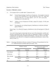
Proportion0 .1 .2 .30 2 4 6 8Number of Childrenmean = 1.939; overdispersion = .2417observed proportionpoisson probneg binom probFigure 3: Negative Binomial and Poisson Fits vs Observed DataWe can further compare the Poisson and negative binomial fit from the null models againstthe observed distribution of counts using nbvargr (download this ado file) as shown in Fig. 3. Wecan see that accounting for the overdispersion also tends to adjust for the excess zeros. Moreover,for these data, the random-effects Poisson/negative binomial regression model appears to fitcounts of 1 more accurately (compare to Fig. 2).Interpreting Random Effects Models. We can think of v as woman-specific unobservedheterogeneity not captured by measured covariates. This random variable may also be viewed indemographic terms as fecundability, in the case of fertility. In mortality research the unobservedmortality propensity is referred to as frailty. Whatever we call it, this captures the dependence inthe individual (Bernoulli) events that contribute to the observed counts. An average value of v is1.0. Values below (above) 1.0 suggest lower (higher) fertility propensity. We have assumed amean of 1.0 for this variable and the model has estimated the variance in its distribution.Because, in principle, each subject has a specific value of unobserved heterogeneity, the estimateof the β’s must be interpreted conditional on the random effects in the population. When thevariance in unobserved heterogeneity is large the coefficients can differ considerably from those ofthe unconditional model. In this case the variance in unobserved heterogeneity is small, so theestimates resemble those in the unconditional model. However, it should be remembered thatestimates are conditional on an unmeasured subject-level variable, so they should not beinterpreted in the same way as those from the standard Poisson regression model, which areunconditional or population average estimates.A remaining question is whether it would be possible to obtain an estimate of a particularwoman’s fertility propensity given her data. After estimating the model, we know somethingabout the distribution of the random effects (at least according to the prior distribution we haveassumed). The Bayesian paradigm is useful for addressing questions about particular values ofthe random effects. Specifically, given a gamma prior distribution on v, g(v), and the likelihood ofthe data conditional on v, f(y|v), the posterior distribution of v isp(v|y) ∝ g(v)f(y|v)With this information, it is possible to obtain the conditional expectation needed to answer the13