Notes on Poisson Regression and Some Extensions

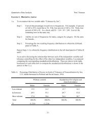
Pr(Y=y)0 .1 .2 .30 2 4 6 8yFigure 2: Comparison of Zero-Inflated Poisson and Poisson and Observed DataandCoding this in Stata is straightforward.scalar ll = e(ll)scalar npar = e(k)scalar nobs = e(N)scalar AIC = -2*ll + 2*nparscalar BIC = -2*ll + log(nobs)*nparscalar list AICscalar list BICBIC = −2 log L + df log nComparing the models we get AIC (BIC) of 5102.2 (5139.4) for the Poisson regression and AIC(BIC) 4963.1 (5032.1) for the zero-inflated model. Lower is better, so the additional work offitting the zero-inflated model is warranted.Nonindependent Events. It is reasonable to expect that there is a certain degree ofdependence between the individual births that constitute a woman’s completed fertility. We canbuild this dependency into the model in a couple of ways. First, we will rewrite the standardmodel as as random effects model with woman-specific unobserved heterogeneity.log(µ i ) = x i β + u iThis should look familiar. The individual-level random effect u has been added to the model, as itwas in the random effects logit models outlined earlier in the course. Statisticians have longrecognized that if a marginal distribution is combined with a particular prior distribution for therandom effect, the resulting distribution is an entirely new distribution. This is the case here, if wespecify a multiplicative factor v that raises or lowers the rate of childbearing for a women in oursample, and assume that it follows a gamma distribution, the resulting marginal distribution is nolonger Poisson, but negative binomial. For example, suppose we consider a multiplicative model.Let’s assume that v is distributed as gamma.µ i = exp(x i β)v iv ∼ gamma(α, β),10