Notes on Poisson Regression and Some Extensions

<strong>Notes</strong> on Poisson Regression and Some ExtensionsDan Powers Soc385K Fall 07Poisson Regression. The Poisson distribution is the most common probability distribution forcount data. The Poisson probability model is appropriate for events that occur randomly overtime and/or space. The probability function for Y is given byPr(Y = y|µ) = e−µ µ yy!y ≥ 0, µ > 0 (1)Usually, we will be interested in estimating µ from the data. For example, an ML estimate is thevalue of µ that is most consistent with the observed data. This estimate is particularly easy tofind for a model without covariates. It is simply the mean count. For example, the number ofoutbreaks of strikes per week in the U.K. from 1948-1949 follows a Poisson distribution.Table 1: Distribution of Major Strikes in the U.K., 1948-59, by Number of Outbreaks per Week.No. Outbreaks/Wk. Observed Expected0 252 2551 229 2292 109 1033 28 314+ 8 7Totals 626 626χ 2 4 = 0.807, p = 0.94The mean number of strikes in the 626 week observation period is ̂µ = 0.899 (taking 4+ = 4).The expected frequencies are generated as N × Pr(Y = y), where ̂µ is substituted in theexpression in Eq. 1.Poisson Sampling Assumptions.• We must be able to divide time or space, usually denoted t, into a large number of subintervalssuch that the probability of occurrence of an event in each of these subintervals is very small.• The probability of the event in each of the subintervals is constant over the time period beingconsidered.• The probability of two or more event occurrences in each/any subinterval must be smallenough to be ignored.• The occurrence or nonoccurrence of an event in one interval must not affect the event occurrenceor nonoccurrence in any other subinterval.1

Moments.var(Y ) = µE(Y ) = µThe mean rateThe variance mean identityHow well does the mean/variance equivalence hold in the example data above? Obtain theobserved proportions of counts and apply the usual formula for the mean and variance of arandom variable. We find, as before, E(Y ) = 0.899 and var(Y ) = 0.860, which are close enoughfor most government work.Models and Estimation.We usually let µ depend on data through a loglinear model , so thatlog(µ i ) = x ′ iβThe log likelihood is written aslog L =n∑ {x′i β − exp(x ′ iβ) − log Γ(y i + 1) }i=1We can ignore the last term in this expression as it does not involve parameters. In other words,the log L evaluated without this term differs from the log L above by an additive constant that isindependent of the model parameters.Exercise 1: Suppose we are interested in finding the MLE of µ (i.e., without covariates). Showthat the log likelihood is simplyn∑log L = log µ y i − nµand that the MLE is ̂µ = ∑ y i /n by solving the first-order conditions for an MLE.Exercise 2: Use the second-order conditions for a maximum to show that the variance of̂µ = ̂µ 2 / ∑ y i .Exercise 3: Develop a least-squares estimator for µ by (1) devising a appropriate loss function(i.e., sum of squared deviations around the expected value), and (2) solving the normal equationfor µ.i=1Numerical Methods. (Please skip this if you are not interested in gory details underlying theblack box of most statistical programs.) The score vector and Hessian matrix areandu = X ′ (y − m)H = −X ′ MX,where m = exp(x ′ îβ) and M = diag(m)We can apply Newton-Raphson or IRLS to this problem. The NR iteration steps arêβ (t) = ̂β (t−1) [− H (t−1)] −1U (t−1) .2

IRLS uses a weighted regression of ẑẑ i = ̂η i + (y i − ̂m i )/ ̂m i ,where ̂η i = x ′ îβ and the iterative weights are ̂m i = exp(̂η i ). All quantities (except y) are updatedat each iteration.Interpretation. The exponentiated model parameters exp(β) are interpreted as multiplicativeeffects on the rate. For a given coefficient pertaining to a unit change in a variable x, valuesgreater than 1 raise the expected rate; values less than 1 lower the expected rate; values equal to1 have no impact on the expected rate.Examples. The following examples show results from models for number of children born for asample of women as a function of several covariates. A first step is to examine the data. Here weare using the GSS. Let’s determine the overall mean childbearing rate by fitting a null modelusing the glm procedure or poisson. Note the technique used to get baseline rate, or theexponentiated effect of the constant term.Null Model.. * NULL model. gen cons = 1. glm childs cons, nocons f(p)Generalized linear models No. of obs = 1501Optimization : ML Residual df = 1500Scale parameter = 1Deviance = 2430.731764 (1/df) Deviance = 1.620488Pearson = 2146.818275 (1/df) Pearson = 1.431212Variance function: V(u) = u[Poisson]Link function : g(u) = ln(u) [Log]AIC = 3.68491Log likelihood = -2764.524679 BIC = -8540.098------------------------------------------------------------------------------| OIMchilds | Coef. Std. Err. z P>|z| [95% Conf. Interval]-------------+----------------------------------------------------------------cons | .6623651 .0185344 35.74 0.000 .6260383 .6986919------------------------------------------------------------------------------. glm, eform------------------------------------------------------------------------------| OIMchilds | IRR Std. Err. z P>|z| [95% Conf. Interval]-------------+----------------------------------------------------------------cons | 1.939374 .0359452 35.74 0.000 1.870187 2.01112------------------------------------------------------------------------------3

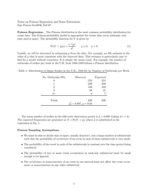
Pr(Y=y)0 .1 .2 .30 2 4 6 8yFigure 1: Comparison of Poisson Model µ = 2 and Observed Data. poisson childs cons, noconsPoisson regression Number of obs = 1501Wald chi2(1) = 1277.14Log likelihood = -2764.5247 Prob > chi2 = 0.0000------------------------------------------------------------------------------childs | Coef. Std. Err. z P>|z| [95% Conf. Interval]-------------+----------------------------------------------------------------cons | .6623651 .0185344 35.74 0.000 .6260383 .6986919------------------------------------------------------------------------------. poisson, irrchilds | IRR Std. Err. z P>|z| [95% Conf. Interval]-------------+----------------------------------------------------------------cons | 1.939374 .0359452 35.74 0.000 1.870187 2.01112------------------------------------------------------------------------------We find that the average number of kids is roughly 2. Suppose we take this rate as the theoreticalmean rate in the population. We can generate a Poisson distribution under this assumption andcompare to the observed distribution as shown in Figure 1. Below are the Stata commands to dothis.gen y = childsmatrix bpois = e(b)gen lampois = exp(bpois[1,1])scalar lampois = 2* generate the predicted distribution for this value of lambda* and plot against empirical distributiongen PrY_pois = exp(-lampois)*lampois^y/exp(lngamma(y+1))twoway (histogram y, discrete fraction blcolor(black) bfcolor(none) ///legend(off) ytitle(Pr(Y=y)) ) (connected PrY_pois y, sort legend(off))A listing of the distribution might also useful for comparison to the theoretical distributionµ = 2.4

. tab yy | Freq. Percent Cum.------------+-----------------------------------0 | 359 23.92 23.921 | 266 17.72 41.642 | 404 26.92 68.553 | 247 16.46 85.014 | 128 8.53 93.545 | 48 3.20 96.746 | 20 1.33 98.077 | 8 0.53 98.608 | 21 1.40 100.00------------+-----------------------------------Total | 1,501 100.00. tab y, sum(PrY_pois) mean| Summary of| PrY_poisy | Mean------------+------------0 | .143793971 | .278870252 | .270416833 | .174813094 | .084756995 | .032875096 | .010626187 | .002944028 | .00071369------------+------------Total | .19380861Incidentally, the estimated mean and variance of y are respectively 1.94 and 2.79, suggesting adeparture from the usual Poisson sampling assumptions.Full Model. Next we add several covariates to the model. For example, coho10 is a linear effectof 10-year birth cohort to capture secular trends toward fewer children among later birth cohorts;married is a dummy variable to capture the tendency for women to postpone childbearing untilafter marriage. 1 The models also control for respondent’s education, income and race.. xi:glm childs coh10 married i.deg nonwht income, family(p)i.deg _Ideg_1-3 (naturally coded; _Ideg_1 omitted)Generalized linear models No. of obs = 1496Optimization : ML Residual df = 1489Scale parameter = 1Deviance = 1934.104383 (1/df) Deviance = 1.298928Pearson = 1661.586326 (1/df) Pearson = 1.1159081 Note that this measure reflects current marital status, not necessarily the marital status at the time of childbearing.5

Variance function: V(u) = u[Poisson]Link function : g(u) = ln(u) [Log]AIC = 3.369277Log likelihood = -2513.219143 BIC = -8951.305------------------------------------------------------------------------------| OIMchilds | Coef. Std. Err. z P>|z| [95% Conf. Interval]-------------+----------------------------------------------------------------coh10 | -.1780332 .0107876 -16.50 0.000 -.1991765 -.15689married | .3857223 .0408991 9.43 0.000 .3055616 .4658831_Ideg_2 | -.161813 .051968 -3.11 0.002 -.2636684 -.0599575_Ideg_3 | -.4039166 .0623524 -6.48 0.000 -.5261251 -.2817081nonwht | .2701722 .0450656 6.00 0.000 .1818453 .3584991income | -.0279788 .0080084 -3.49 0.000 -.043675 -.0122826_cons | 2.229226 .100984 22.08 0.000 2.031301 2.427151------------------------------------------------------------------------------. glm, eform------------------------------------------------------------------------------| OIMchilds | IRR Std. Err. z P>|z| [95% Conf. Interval]-------------+----------------------------------------------------------------coh10 | .8369146 .0090283 -16.50 0.000 .8194053 .8547981married | 1.470676 .0601493 9.43 0.000 1.357387 1.593421_Ideg_2 | .8506003 .044204 -3.11 0.002 .7682282 .9418045_Ideg_3 | .6676998 .0416327 -6.48 0.000 .5908902 .7544939nonwht | 1.31019 .0590445 6.00 0.000 1.199429 1.43118income | .972409 .0077875 -3.49 0.000 .957265 .9877925------------------------------------------------------------------------------. * or another way. xi:poisson childs coh10 married i.deg nonwht income, irri.deg _Ideg_1-3 (naturally coded; _Ideg_1 omitted)Poisson regression Number of obs = 1496LR chi2(6) = 483.99Prob > chi2 = 0.0000Log likelihood = -2513.2191 Pseudo R2 = 0.0878------------------------------------------------------------------------------childs | IRR Std. Err. z P>|z| [95% Conf. Interval]-------------+----------------------------------------------------------------coh10 | .8369146 .0090283 -16.50 0.000 .8194053 .8547981married | 1.470676 .0601493 9.43 0.000 1.357387 1.593421_Ideg_2 | .8506003 .044204 -3.11 0.002 .7682282 .9418045_Ideg_3 | .6676998 .0416327 -6.48 0.000 .5908902 .7544939nonwht | 1.31019 .0590445 6.00 0.000 1.199429 1.43118income | .972409 .0077875 -3.49 0.000 .957265 .9877925------------------------------------------------------------------------------6

. fitstatMeasures of Fit for poisson of childsLog-Lik Intercept Only: -2755.216 Log-Lik Full Model: -2513.219D(1489): 5026.438 LR(6): 483.994Prob > LR: 0.000McFadden’s R2: 0.088 McFadden’s Adj R2: 0.085ML (Cox-Snell) R2: 0.276 Cragg-Uhler(Nagelkerke) R2: 0.284AIC: 3.369 AIC*n: 5040.438BIC: -5858.971 BIC’: -440.131BIC used by Stata: 5077.612 AIC used by Stata: 5040.438The constant implies that the conditional mean rate of childbearing over the life of the sampledwomen is exp(2.23) = 9.293 children. Wow! This seems large, but remember that it is adjusted upor down depending on covariates. Here is a table showing predicted rates by race, marital status,and “boomer” status evaluated at the mean level of income and education. This is actually basedon a different model that distinguishes between those women born before 1950 and those bornbetween 1950 and 1970 (boomer).. prtab married boomer nonwhtpoisson: Predicted rates for childs--------------------------------------------| nonwht and boomer| ------ 0 ----- ------ 1 -----married | 0 1 0 1----------+---------------------------------0 | 2.0372 1.1673 2.5443 1.45791 | 2.8994 1.6614 3.6211 2.0749--------------------------------------------boomer married _Ideg_2 _Ideg_3 nonwht incomex= .60093583 .46657754 .5447861 .31149733 .22393048 10.695856The income effect is −0.028, and income is measured in $2500 increments, so a $2500 increase inincome brings about a exp(−0.028) = 0.97 change in the number of children.Exercise 4: Show that this is a 3% reduction in the rate per $2500 increase in income. Show thatmarriage increases the rate by 47%.Zero Inflated Poisson Data. Our data could contain an excess of zeros. By this we meanthat there are some zeros that would occur naturally but that the data could contain more zerosthan would be expected under Poisson sampling. The excess zeros will affect the mean andvariance. In particular, the mean/variance equivalence will no longer hold. For example, themean number of children in the U.S. is about 2 children per family. We can compare this to ourobserved distribution (Fig. 1). However, we find that the unconditional Poisson model does notpredict the zeros as well as it predicts the other values. In this case, we may want to test thezero-inflated Poisson model against the standard model.7

The probability function for zero-inflated count variable Y z can be specified as,⎧⎨p + (1 − p)e −µ if y = 0Pr(Y z = y|p, µ) =⎩(1 − p) e−µ µ yy!if y > 0(2)Unlike the Poisson distribution which is determined by a single parameter, µ, the ZIP distributionis determined by two parameters µ (i.e., the parameter for the standard Poisson distribution) andp (i.e., the probability of being an inflated zero). The mean and variance of a zero-inflated countvariable are, respectively,E(Y z ) = µ(1 − p)andvar(Y z ) = µ(1 − p)(1 + µp),which shows the nature of the overdispersion via the mean to variance ratio when count data arecharacterized by an excess of 0’s. The variance is (1 + µp) times the mean.Estimation.We can model the inflated-zero probability as a function of covariates,and the Poisson rates as,The likelihood function can then be written as,p i = exp(x′ i α)1 + exp(x ′ i α),µ i = exp(x ′ iβ).log L =n∑log p i + (1 − p i ) exp(µ i ) + log{(1 − p i ) exp(−µ i )} + yµ i − log Γ(y i + 1). (3)i=1Interpretation. Interpretation of the results from this model is straightforward. We caninterpret the parameters in the inflated portion as effects on the log odds of being zero. 2 Theother parameters have the usual Poisson regression interpretation. Using results from the nullmodel and applying the formulas above for the mean and variance, we get ̂µ = e 0.829 (0.846),which is 1.94 for the mean, where ̂α = −1.7069, so p = 0.153. Using the formula above, thevariance is 2.621. The mean is exactly reproduced by the model, the variance is closer to theestimate of 2.79 from the raw data than was the estimate from the Poisson regression model.Example.Zero-inflated poisson regression Number of obs = 1496Nonzero obs = 1140Zero obs = 356Inflation model = logit LR chi2(6) = 180.92Log likelihood = -2468.552 Prob > chi2 = 0.00002 Other probability distributions for zero-inflation are possible.8

------------------------------------------------------------------------------childs | Coef. Std. Err. z P>|z| [95% Conf. Interval]-------------+----------------------------------------------------------------childs |boomer | -.4280169 .0415171 -10.31 0.000 -.509389 -.3466449married | .0851949 .0454331 1.88 0.061 -.0038523 .1742421_Ideg_2 | -.2272821 .0532389 -4.27 0.000 -.3316285 -.1229357_Ideg_3 | -.4033855 .0640953 -6.29 0.000 -.5290099 -.2777611nonwht | .1115982 .0490869 2.27 0.023 .0153897 .2078068income | -.0271459 .0083784 -3.24 0.001 -.0435673 -.0107244_cons | 1.473333 .0846589 17.40 0.000 1.307404 1.639261-------------+----------------------------------------------------------------inflate |boomer | 1.486534 .2721459 5.46 0.000 .9531378 2.01993_Ideg_2 | .0095591 .3414682 0.03 0.978 -.6597061 .6788244_Ideg_3 | .7008029 .355765 1.97 0.049 .0035162 1.39809nonwht | -1.289767 .3455102 -3.73 0.000 -1.966955 -.6125796_cons | -2.027314 .3265346 -6.21 0.000 -2.66731 -1.387317------------------------------------------------------------------------------Here we find that having less than a HS education ( Ideg 2) has a negligible effect on beingchildless, but a large effect on the rate of childbearing. We can use BIC/AIC criteria to check thismodel against the Poisson regression model (these are not nested). It is worthwhile to examinehow well it fits the observed distribution compared to the Poisson model. Fig. 2 examines the nullmodel of each specification. Below is the code to make the graph.*do Poisson Assumptions hold?* zero inflation NULL model accounts for excess 0 counts --> compare to Poisson NULL model*gen cons = 1zip childs, inflate(cons)matrix bzip = e(b)gen lamzip = exp(bzip[1,1])gen p1 = exp(bzip[1,2])/(1 + exp(bzip[1,2]))gen p0 = 1 - p1gen PrY_zip = p1 + p0*( exp(-lamzip)*lamzip^y/exp(lngamma(y+1)) ) if y==0replace PrY_zip = p0*( exp(-lamzip)*lamzip^y/exp(lngamma(y+1)) ) if (y ~=0)twoway (histogram y, discrete fraction blcolor(black) bfcolor(none) ///legend(off) ytitle(Pr(Y=y)) ) (connected PrY_pois y, sort legend(off)) ///(connected PrY_zip y, sort legend(off))There is always the question of which variables should appear in each section of the zip model.It is best to retain the complete model specification in the Poisson part and attempt to justify(theoretically) which variables should should be predictive of zeros, and included in the zeroinflation portion of the model. Then we can trim the model accordingly based on significancetests. How well does this model compare to the standard Poisson model. They are not nested, sowe should use other ad-hoc criteria such as AIC or BIC. We can use Long and Freese fitstatroutine. However, it is not hard to do this by hand. First, we need a definition. There are severalversion of these statistics. Here we adopt one that is on the same scale as −2 log L. Both of thesefit statistics provide penalties for over fitting the model. In the case of BIC, there is a sample sizepenalty also.AIC = −2 log L + 2df9

Pr(Y=y)0 .1 .2 .30 2 4 6 8yFigure 2: Comparison of Zero-Inflated Poisson and Poisson and Observed DataandCoding this in Stata is straightforward.scalar ll = e(ll)scalar npar = e(k)scalar nobs = e(N)scalar AIC = -2*ll + 2*nparscalar BIC = -2*ll + log(nobs)*nparscalar list AICscalar list BICBIC = −2 log L + df log nComparing the models we get AIC (BIC) of 5102.2 (5139.4) for the Poisson regression and AIC(BIC) 4963.1 (5032.1) for the zero-inflated model. Lower is better, so the additional work offitting the zero-inflated model is warranted.Nonindependent Events. It is reasonable to expect that there is a certain degree ofdependence between the individual births that constitute a woman’s completed fertility. We canbuild this dependency into the model in a couple of ways. First, we will rewrite the standardmodel as as random effects model with woman-specific unobserved heterogeneity.log(µ i ) = x i β + u iThis should look familiar. The individual-level random effect u has been added to the model, as itwas in the random effects logit models outlined earlier in the course. Statisticians have longrecognized that if a marginal distribution is combined with a particular prior distribution for therandom effect, the resulting distribution is an entirely new distribution. This is the case here, if wespecify a multiplicative factor v that raises or lowers the rate of childbearing for a women in oursample, and assume that it follows a gamma distribution, the resulting marginal distribution is nolonger Poisson, but negative binomial. For example, suppose we consider a multiplicative model.Let’s assume that v is distributed as gamma.µ i = exp(x i β)v iv ∼ gamma(α, β),10

such that E(v) = α/β and var(v) = α/β 2 . In Bayesian terms, the gamma distribution is theconjugate prior distribution for the Poisson (and other distributions in the exponential family).When the prior distribution is combined with the Poisson distribution for y, conditional on v, theresulting unconditional distribution (or posterior distribution) of y is negative binomial. This wasdiscovered not long after the Poisson distribution, perhaps round 1909.For convenience, we normalize the distribution of v so that it has a mean of 1.0 as follows:E(v) = 1.0and this implies,so the resulting distribution for v isvar(v) = 1/α,g(v) = αα v α−1Γ(α)exp(−αv) α > 0The likelihood of y for the ith woman conditional on her random effect v i is.L(y i |v i )To obtain the marginal likelihood of y for the whole sample, we need to integrate over thedistribution of v for each woman in our sample in order to “average” out the random effect.L m = ∏ ∫L(y i |v i )g(v)dvivThe resulting distribution can be evaluated in closed formL m = ∏ iΓ(y i + 1 α ) [αµ] i yi[1] 1αΓ(y i + 1)Γ( 1 α ) 1 + αµ i 1 + αµ iExercise 5. Derive the negative binomial distribution as a mixture of a Poisson and gammadistribution.A negative binomial variable has mean E(Y ) = µ and variance var(Y ) = µ + µα −1 . The loglikelihood function for this model is,log L =n∑log(1 − α) − log(1 + αy i ) + y i log µ i − (y + 1 α ) log(1 − αµ i) − log Γ(y i + 1).i=1It is a bit more difficult to optimize this model, but it is straightforward. All major statisticalsoftware (SAS, R, Stata have routines for estimating this model.Estimation. We maximize this likelihood with respect to the parameters β and α, theoverdispersion parameter. This is the standard deviation of the gamma-distributed random effectmentioned earlier (note that we have assumed this effect to have a mean of 1 and have estimatedits variance using the current sample of women). In fact, the negative binomial is identical to anindividual-level random-effects Poisson regression. We get identical results using either nbreg orxtpois, however we must supply a respondent ID number in order to identify the clusters (eachof size 1) to be used in the random effects specification.11

. nbreg childsNegative binomial regression Number of obs = 1501LR chi2(0) = 0.00Prob > chi2 = .Log likelihood = -2710.1185 Pseudo R2 = 0.0000------------------------------------------------------------------------------childs | Coef. Std. Err. z P>|z| [95% Conf. Interval]-------------+----------------------------------------------------------------_cons | .6623651 .0224627 29.49 0.000 .618339 .7063912-------------+----------------------------------------------------------------/lnalpha | -1.419918 .1278525 -1.670504 -1.169331-------------+----------------------------------------------------------------alpha | .2417339 .0309063 .1881522 .3105746------------------------------------------------------------------------------Likelihood-ratio test of alpha=0: chibar2(01) = 108.81 Prob>=chibar2 = 0.000. gen idnum = _n. xtpois childs, i(idnum)Random effects u_i ~ Gamma Obs per group: min = 1avg = 1.0max = 1Wald chi2(0) = .Log likelihood = -2710.1185 Prob > chi2 = .------------------------------------------------------------------------------childs | Coef. Std. Err. z P>|z| [95% Conf. Interval]-------------+----------------------------------------------------------------_cons | .6623651 .0224627 29.49 0.000 .618339 .7063912-------------+----------------------------------------------------------------/lnalpha | -1.419918 .1278525 -1.670504 -1.169331-------------+----------------------------------------------------------------alpha | .2417339 .0309063 .1881522 .3105746------------------------------------------------------------------------------Likelihood-ratio test of alpha=0: chibar2(01) = 108.81 Prob>=chibar2 = 0.000The test on the alpha parameter is a test of overdispersion. This suggests an improved fit fromthis model. The variance of the random effect v is 0.24 2 (given by alpha). As this goes to 0, themodel approaches the usual Poisson regression model. In fact, here the results do not changemuch from the original model. Note that the alpha in the Stata output is not the same α fromthe gamma distribution. Recall that the α parameter from the gamma distribution is thereciprocal of the variance of the random effect, i.e., the reciprocal of the quantity reported asalpha by Stata, or 4.14. recall that the observed mean and variance of y are, respectively, 1.94and 2.79. Under the negative binomial regression model, the estimated mean is the same and thevariance is ̂µ + ̂µ/α = 1.94 + 1.94(0.242) = 2.41, which is getting a good deal closer to 2.79.Likelihood ratio tests can also be carried out of the current model against the null model. Thelog L from the corresponding Poisson regression model is −2764.52 compared to a log L of−2710.12 for the negative binomial model. The likelihood ratio χ 2 for is 108.81 with 1 df, whichis exactly what is reported in the output. Note that the standard errors are larger than in theoriginal Poisson regression model due to this adjustment to the model, so more conservativesignificance tests will follow.12

Proportion0 .1 .2 .30 2 4 6 8Number of Childrenmean = 1.939; overdispersion = .2417observed proportionpoisson probneg binom probFigure 3: Negative Binomial and Poisson Fits vs Observed DataWe can further compare the Poisson and negative binomial fit from the null models againstthe observed distribution of counts using nbvargr (download this ado file) as shown in Fig. 3. Wecan see that accounting for the overdispersion also tends to adjust for the excess zeros. Moreover,for these data, the random-effects Poisson/negative binomial regression model appears to fitcounts of 1 more accurately (compare to Fig. 2).Interpreting Random Effects Models. We can think of v as woman-specific unobservedheterogeneity not captured by measured covariates. This random variable may also be viewed indemographic terms as fecundability, in the case of fertility. In mortality research the unobservedmortality propensity is referred to as frailty. Whatever we call it, this captures the dependence inthe individual (Bernoulli) events that contribute to the observed counts. An average value of v is1.0. Values below (above) 1.0 suggest lower (higher) fertility propensity. We have assumed amean of 1.0 for this variable and the model has estimated the variance in its distribution.Because, in principle, each subject has a specific value of unobserved heterogeneity, the estimateof the β’s must be interpreted conditional on the random effects in the population. When thevariance in unobserved heterogeneity is large the coefficients can differ considerably from those ofthe unconditional model. In this case the variance in unobserved heterogeneity is small, so theestimates resemble those in the unconditional model. However, it should be remembered thatestimates are conditional on an unmeasured subject-level variable, so they should not beinterpreted in the same way as those from the standard Poisson regression model, which areunconditional or population average estimates.A remaining question is whether it would be possible to obtain an estimate of a particularwoman’s fertility propensity given her data. After estimating the model, we know somethingabout the distribution of the random effects (at least according to the prior distribution we haveassumed). The Bayesian paradigm is useful for addressing questions about particular values ofthe random effects. Specifically, given a gamma prior distribution on v, g(v), and the likelihood ofthe data conditional on v, f(y|v), the posterior distribution of v isp(v|y) ∝ g(v)f(y|v)With this information, it is possible to obtain the conditional expectation needed to answer the13

question above.∫vE(v|y) = ∫vg(v)f(y|v)dvv g(v)f(y|v)dvThis is referred to the expected a-posteriori estimate of the random effect, or empirical Bayesestimate for short. In many cases this expression would have to be solved numerically, or othermethods might need to be used to evaluate it. It turns out to be convenient that that a gammaprior was used. In this case, the posterior distribution is also gamma, but with shape parameterα + y i and scale parameter α + µ. If we had observed j multiple events on the same individual orcounts among clusters of j dependent units of analysis, the shape and scale parameters would beα + ∑ j y ij and α + ∑ j µ ij. Thus, in the case of these types of data structures, we have amultilevel Poisson model. 3Next we fit the full model. Note that the estimated variance in the random effect is 0.073,which implies almost no variation in the random effect distribution. A proportionate reduction inerror statistic can be computed to compare the change in the proportion of variance explained bythis model (indexed by 1) compared to the null model (indexed by 0).R 2 p = var(v) 0 − var(v) 1var(v) 0= 0.242 − 0.073.242 = 0.698This suggests that about 70% of the variance in number of children is accounted for by thewoman-specific variables included in the full model. To gauge the correlation in the individualevents contributing to total fertility we can construct a measure a measure asICC =var(u)var(u) + var(y) = 0.0730.073 + 2 = 0.035which is not much. These kinds of random effects models are much more useful when we haverepeated measures on the same set of respondents (i.e., panel data) or clustered counts data fromindividuals nested in wider contexts (fertility of siblings etc.).Random-effects Poisson regression Number of obs = 1496Log likelihood = -2537.2144 Prob > chi2 = 0.0000------------------------------------------------------------------------------childs | Coef. Std. Err. z P>|z| [95% Conf. Interval]-------------+----------------------------------------------------------------boomer | -.5613786 .041419 -13.55 0.000 -.6425583 -.4801989married | .3626 .0438245 8.27 0.000 .2767055 .4484945_Ideg_2 | -.2270964 .055744 -4.07 0.000 -.3363527 -.1178401_Ideg_3 | -.4895984 .065998 -7.42 0.000 -.6189521 -.3602448nonwht | .2258126 .0484695 4.66 0.000 .1308141 .3208111income | -.0287399 .008614 -3.34 0.001 -.045623 -.0118567_cons | 1.291956 .0876294 14.74 0.000 1.120205 1.463706-------------+----------------------------------------------------------------/lnalpha | -2.615761 .3047629 -3.213085 -2.018436-------------+----------------------------------------------------------------alpha | .0731122 .0222819 .0402323 .1328631------------------------------------------------------------------------------Likelihood-ratio test of alpha=0: chibar2(01) = 13.78 Prob>=chibar2 = 0.0003 This differs from the usual multilevel models that assume normal or multivariate normal random effects.14

Density0 1 2 3 4 5.8 1 1.2 1.4vhat1Figure 4: Distribution of Empirical Bayes Estimates of Random EffectThe distribution of random effects from this model can be shown a couple of ways. A graphicalrepresentation is given in Fig. 4. The commands to fit the model and compute the subject-specificrandom effect estimates are given below.xi: xtpois childs boomer married i.deg nonwht income, i(idnum)xtpois, irrpredict xb, xbgen lambda1 = exp(xb)scalar alpha = 1/(exp([lnalpha]_cons))gen vhat1 = (y + alpha)/(lambda1 + alpha)sum vhat1, detailhistogram vhat1-------------------------------------------------------------vhat1-------------------------------------------------------------Percentiles Smallest1% .822471 .75523535% .8726416 .780816610% .8964401 .7998554 Obs 149625% .9296511 .8005092 Sum of Wgt. 149650% .9884257 Mean 1Largest Std. Dev. .094407175% 1.053683 1.38304790% 1.123672 1.383047 Variance .008912795% 1.170076 1.420766 Skewness .803510299% 1.288011 1.431209 Kurtosis 4.09398Thus, based on this data, the propensity for childbearing (net of covariates) is about 1.25 timeshigher for women at the 90% percentile of the random effects distribution relative to those at the10th percentile, which is not much of a difference.Extensions. It is also possible to combine both zero-inflation with the negative binomialdistributional assumption. What you get, of course, is the zero-inflated negative binomial model(zinb). There are many extensions of these extensions that have not made their way into canned15

packages. They are very useful for particular applications. When this model is fit to these data,the overdispersion parameter is no longer statistically significant.Exercise 6: Fit a common model specification (i.e., same set of variables) for all these models andcompare on the basis of likelihood ratio tests (when possible) and BIC criteria (for non-nestedmodels). Which model emerges as best for this data.Models for Rates in Time. Let t 1 , t 2 , . . . , t n denote the waiting times until an event occursfor a sample of n individuals, with distribution function F (t) = Pr(T < t) and probability densityfunction f(t), where we assume that T is a continuous random variable (T > 0). The hazard rate,intensity function, or failure rate is denoted by µ(t). The hazard rate is the instantaneousprobability of an event in the interval [t, t + ∆t], given that the event has not already occurredbefore the beginning of the interval. More formally, the hazard rate is the limit of a conditionalprobability (or transition probability)1µ(t) = lim Pr[t ≤ T < t + ∆t | T ≥ t]. (4)∆t→0 ∆t∆t>0The probability of surviving the interval [t, t + ∆t] is given by the survival function.S(t) = Pr[T > t] = 1 − F (t) =∫ ∞tf(u)du. (5)If we assume that the random variable for waiting-time (T ) follows an exponential distributionwith density function, f(t) = µ exp(−µt), the expressions for the survival function in Eq. 5 isS(t) = exp(−µt). The expression for the hazard rate of Eq. 4 is defined is the ratio, µ(t) =f(t)/S(t) = µ. For the exponential distribution, this implies a constant hazard over time (i.e., notdepending on t).Consider a Poisson variate d that denotes the number of events occurring in an observationwindow (exposure period) of length t. If events can occur repeatedly over time, and if the timesbetween events are independent exponential variables with mean time to event occurrence is givenby E(T ) = 1/µ (i.e., a time-homogeneous Poisson process), then the probability of d events in atime-interval of length t follows a Poisson distribution,Pr(d | µ, t) = (tµ)d exp(−tµ). (6)d!The mean number of events in time-interval t is, λ = tµ. For a sample of size n, we can model theconditional mean count as a function of independent variables, so that for the ith individual, theexpected number of events in time-interval t i isµ i = t i λ i = t i exp(x ′ iβ).The likelihood is a product of the individual Poisson probabilities in Eq. 6, and is proportional toL =n∏(t i λ i ) d iexp(−t i λ i ), (7)i=1which is the kernel of a Poisson likelihood.It will often be the case that we do not observe the event times for some individuals in thesample. In this case, the event times are said to be right censored, and the Poisson variate is16

coded 0, otherwise it is coded 1 (event). Consider the likelihood for an exponential model, whichis appropriate for the random variable T , and deals with censoring.L ==n∏i=1λ d iiexp(−t i λ i )n∏exp(x ′ iβ) d iexp{−t i exp(x ′ iβ)}.i=1(8)It turns out that maximizing the Poisson likelihood of Eq. 7 yields the same MLEs as maximizingthe the exponential likelihood in Eq. 8. 4 This can be seen by rewriting Eq. 8 in a somewhatdifferent form asL =n∏n∏(t i λ i ) d iexp(−t i λ i )/i=1i=1t d ii . (9)The term in the denominator of Eq. 9 does not depend on unknown parameters and can beignored in estimation. 5 This implies that the exponential hazard rate model can be estimatedusing a Poisson regression model for counts. Taking logs of the Poisson mean (µ i = t i λ i ), weobtain the following loglinear modellog µ i = log t i + log λ i= log t i + x ′ iβ.(10)The term, log t i appearing in this model has a fixed coefficient of one and is known as an “offset.”To fit these models using software for Poisson regression, we declare the log exposure as an offsetterm in the model. The table below shows the cumulative proportion surviving (i.e., notexperiencing) an event (premarital birth) by a particular age. Respondents can be removed fromrisk of this event through marriage. In this case, by age 20, about 20 percent of the sample hasexperienced a premarital birth; by age 35 about 45% have.. ltable agecens pbirBeg.Std.Interval Total Deaths Lost Survival Error [95% Conf. Int.]-------------------------------------------------------------------------------14 15 1345 8 1 0.9940 0.0021 0.9881 0.997015 16 1336 19 3 0.9799 0.0038 0.9708 0.986216 17 1314 41 10 0.9492 0.0060 0.9360 0.959717 18 1263 51 20 0.9106 0.0078 0.8939 0.924718 19 1192 46 68 0.8744 0.0092 0.8552 0.891219 20 1078 49 82 0.8331 0.0105 0.8114 0.852520 21 947 44 66 0.7930 0.0116 0.7692 0.814621 22 837 34 80 0.7591 0.0124 0.7337 0.782522 23 723 21 91 0.7356 0.0131 0.7090 0.760223 24 611 20 85 0.7097 0.0138 0.6816 0.735924 25 506 15 65 0.6873 0.0146 0.6577 0.714825 26 426 6 39 0.6771 0.0149 0.6469 0.705426 27 381 7 42 0.6639 0.0154 0.6327 0.693227 28 332 11 63 0.6396 0.0165 0.6062 0.671028 29 258 8 60 0.6172 0.0177 0.5814 0.65094 The d! term appearing in the denominator does not depend on unknown parameters, so it can be effectivelyignored for estimating β.5 For the statistical relationship to hold, the events must correspond to n independent, time-homogeneous Poissonprocesses with rates, λ i. The number of events for the ith process in a time interval of length t follows a Poissondistribution with mean t i λ i . The observed number of events (d i ) is not 0,1,2,3,. . ., but 0 or 1. This is equivalent toobserving the ith process until either a first event occurs, or a fixed time, t i, has elapsed without the event occurring.17

29 30 190 4 49 0.6023 0.0188 0.5643 0.638130 31 137 2 35 0.5922 0.0198 0.5523 0.629831 32 100 3 36 0.5705 0.0227 0.5248 0.613632 33 61 2 31 0.5455 0.0278 0.4894 0.598033 34 28 0 16 0.5455 0.0278 0.4894 0.598034 35 12 0 11 0.5455 0.0278 0.4894 0.598035 36 1 0 1 0.5455 0.0278 0.4894 0.5980-------------------------------------------------------------------------------We can use the methods described above to analyze individual data like these. We can obtaingood results using log linear models for tables. Consider the following table of race by age ofevent (agecat = 1 if < 20, 2 otherwise ) that was derived from these data.. list race agecat D T+------------------------------------+race agecat D T--------------------------------------1. Hispanic 1 31 5082.682. Hispanic 2 36 896.433. Black 1 143 8252.044. Black 2 103 1336.375. White 1 40 12801.896. White 2 38 2773.93+------------------------------------+The variables D i and R i denote the number of events in each category and the person years ofexposure to risk for the subjects in that category. The empirical rates are then. We assume D i tobe a Poisson variable with mean µ i . Using the covariates agecat and race as x, we can write aloglinear model in log µ ilog(µ i )λ i R i = x ′ iβ + log R iwith log R i as an “offset” term whose coefficient is fixed at 1.. xi: glm D i.agecat i.race, f(p) offset(logT)Generalized linear models No. of obs = 6Optimization : ML: Newton-Raphson Residual df = 2Scale parameter = 1Deviance = 2.167700605 (1/df) Deviance = 1.08385Pearson = 2.176320642 (1/df) Pearson = 1.08816Variance function: V(u) = u[Poisson]Link function : g(u) = ln(u) [Log]Standard errors : OIMLog likelihood = -18.57892505 AIC = 7.526308BIC = -1.415818333------------------------------------------------------------------------------D | Coef. Std. Err. z P>|z| [95% Conf. Interval]-------------+----------------------------------------------------------------_Iagecat_2 | 1.557508 .1017639 15.31 0.000 1.358055 1.756962_Irace_2 | .8540021 .1378224 6.20 0.000 .5838751 1.124129_Irace_3 | -.870819 .1666529 -5.23 0.000 -1.197453 -.5441853_cons | -4.937157 .1306748 -37.78 0.000 -5.193275 -4.68103918

logT | (offset)------------------------------------------------------------------------------The baseline rate of premarital birth is exp(−4.937) = 0.007 or about 7 premarital births perthousand per year of age (after age 11). This event is exp(1.557) = 4.74 time higher for womenover the age of 20. The comparison category for race is Hispanic, so we find rates that are about58% lower for whites and about 2.34 times higher for blacks at any age (relative to Hispanics).Because the rates are proportionally higher or lower depending on the values of the covariates inthe model, this model is referred to as a proportional hazards model.Exercise 7: Using the table above, fit a model that allows the risk to vary by race depending onage. That is, fit a model in which there are nonproportional effects of race and determine if thereis evidence of nonproportionality.Hazard Models with Cluster-level Frailty We can combine ideas from the previoussection to model for events. Suppose we consider a sampling plan that records age at firstpremarital birth for the subsample of white women in the NLSY. The NLSY includes respondentsand up to 6 sibling respondents in the data. We can use this data structure to illustrate multilevelhazard rate models. Duration, t ij denotes the age at first premarital birth for the ith individualin the jth family. The event-status indicator d ij = 1 denotes a premarital birth at time t ij for theith individual in the jth family. A proportional hazard model accounting for cluster-level frailty ish(t ij ) = h 0 (t ij ) exp{x ij (t ij )β}v j ,where we assume that v j follows a gamma distribution with mean 1 and variance φ = 1/α asbefore. The model can be estimated using the EM-algorithm, which treats v j as a known relativerisk. At each EM iteration, our estimate of v j is updated using current results from a loglinearmodel (Poisson regression) and our current estimates of α as follows:̂v j = ̂α + d +ĵα + H +jwhere d +j is the total number of events in the jth cluster and H +j is the sum of the integratedhazards in the jth cluster. The imputed frailties from each iteration are then treated as part ofthe “offset” term in a Poisson regression. The model can also be estimated directly using ML anda Poisson regression model for panel data (xtpois) in Stata.Stata Example Script.set memory 5000#delimit;infile v1 intr v3 d ts tf v7 cid c9 nonintm12 m13 mmed mwrk14 adjinc msinc nsibs southurban fundpro cathol weekly profam selfest test using 6W1.dat;gen offs=log(tf-ts);gen a1 = intr==1;gen a2 = intr==2;gen a3 = intr==3;gen a4 = intr==4;gen a5 = intr==5;19

gen a6 = intr==6;egen id = fill(1 2);xtpois d a1 a2 a3 a4 a5 a6 nonint m12 adjinc nsibssouth urban fundpro cathol profam selfest,offset(offs) i(cid) nocons;Results.Random-effects Poisson Number of obs = 9359Group variable (i) : cid Number of groups = 1936Random effects u_i ~ Gamma Obs per group: min = 1avg = 4.8max = 23Wald chi2(16) = 2679.28Log likelihood = -1144.5603 Prob > chi2 = 0.0000------------------------------------------------------------------------------d | Coef. Std. Err. z P>|z| [95% Conf. Interval]---------+--------------------------------------------------------------------a1 | -4.854541 .8016085 -6.056 0.000 -6.425665 -3.283418a2 | -2.649949 .7782366 -3.405 0.001 -4.175264 -1.124633a3 | -2.143511 .7772958 -2.758 0.006 -3.666983 -.6200393a4 | -2.185339 .779154 -2.805 0.005 -3.712453 -.6582254a5 | -2.053847 .794188 -2.586 0.010 -3.610427 -.4972672a6 | -2.106344 .8363073 -2.519 0.012 -3.745476 -.4672121nonint | .9371541 .1693922 5.532 0.000 .6051515 1.269157m12 | .8770516 .1649014 5.319 0.000 .5538508 1.200252adjinc | -.0000559 .0000168 -3.319 0.001 -.0000889 -.0000229nsibs | .0572207 .0386449 1.481 0.139 -.0185219 .1329633south | -.7573547 .2066934 -3.664 0.000 -1.162466 -.3522431urban | .2083464 .1893081 1.101 0.271 -.1626906 .5793835fundpro | .7688226 .2057846 3.736 0.000 .3654923 1.172153cathol | -.2760485 .1953083 -1.413 0.158 -.6588457 .1067487profam | .5185107 .1837613 2.822 0.005 .158345 .8786763selfest | -1.034571 .1925264 -5.374 0.000 -1.411916 -.6572266offs | (offset)---------+--------------------------------------------------------------------/lnalpha | .2281934 .4508365 -.6554299 1.111817---------+--------------------------------------------------------------------alpha | 1.256328 .5663986 .5192188 3.039876------------------------------------------------------------------------------Likelihood ratio test of alpha=0: chi2(1) = 9.34 Prob > chi2 = 0.0022Imputed Frailties. Suppose you want to know more about the distribution of frailty or wantedto know which observed family-level traits might have an impact on a family’s frailty? 6 Theexpression for ̂v j can be evaluated using Stata as follows:set memory 5000#delimit;6 By assumption, the x’s are uncorrelated with the v’s so statement is contradictory. That is, under our model’sassumptions, frailty should not impact other covariates. However, the variance in frailty could be affected by theinclusion of covariates.20

infile v1 intr v3 d ts tf v7 cid c9 nonintm12 m13 mmed mwrk14 adjinc msinc nsibs southurban fundpro cathol weekly profam selfest test using 6W1.dat;gen offs=log(tf-ts);gen a1 = intr==1;gen a2 = intr==2;gen a3 = intr==3;gen a4 = intr==4;gen a5 = intr==5;gen a6 = intr==6;egen id = fill(1 2);/* Fit baseline hazard and retrieve imputed frailties */xtpois d a1 a2 a3 a4 a5 a6, offset(offs) i(cid) nocons;predict xbeta, xb;gen t = tf - ts;gen Ihaz=t*exp(xbeta - offs);gen a=1/e(alpha);collapse (mean) p = a (rawsum) H=Ihaz (rawsum) D=d, by(cid);gen w = (D+p)/(H+p);summarize w, detail;Here, I let w denote each family’s frailty. We use the collapse command to get the desiredquantities. Note that p corresponds to 1/φ, which is called alpha in Stata. Since it is constantover clusters, we just take the mean. Other quantities H and D correspond to the sum of acluster’s integrated hazards and a cluster’s total number of events. This results in a new data setcontaining cluster-specific frailties. You could also include observed characteristics of the cluster,in order to see how these would affect frailty in a regression model. Since frailty must be > 0, agood model might be a loglinear regression model such as:log v j = x j β + ε.Here, we asked only for the descriptive summary of frailty from a proportional hazards modelthat fits only the baseline hazard. The quantiles are probably most relevant.Log likelihood = -1248.9537 Prob > chi2 = 0.0000------------------------------------------------------------------------------d | Coef. Std. Err. z P>|z| [95% Conf. Interval]---------+--------------------------------------------------------------------a1 | -6.45445 .2405448 -26.833 0.000 -6.925909 -5.982991a2 | -4.282342 .1458461 -29.362 0.000 -4.568195 -3.996489a3 | -3.890296 .1553783 -25.038 0.000 -4.194832 -3.58576a4 | -3.995447 .1894533 -21.089 0.000 -4.366768 -3.624125a5 | -3.816231 .2659806 -14.348 0.000 -4.337543 -3.294918a6 | -3.749099 .3883572 -9.654 0.000 -4.510265 -2.987933offs | (offset)---------+--------------------------------------------------------------------/lnalpha | 1.41132 .3308904 .7627865 2.059853---------+--------------------------------------------------------------------alpha | 4.101364 1.357102 2.144243 7.844815------------------------------------------------------------------------------Likelihood ratio test of alpha=0: chi2(1) = 27.61 Prob > chi2 = 0.0000w21

-------------------------------------------------------------Percentiles Smallest1% .2922498 .18123255% .3799957 .200074810% .4219338 .2040029 Obs 193625% .519807 .2328834 Sum of Wgt. 193650% .6829988 Mean 1Largest Std. Dev. 1.07957475% .8374014 6.5031590% 2.366105 7.647584 Variance 1.1654895% 4.012737 8.142287 Skewness 2.92292699% 4.941901 8.929889 Kurtosis 11.43697Note that empirically the estimated mean frailty is 1 and the variance is 1.165.22