Chapter 8. Inferences from Two Samples ( ) ( ) ( ) ()

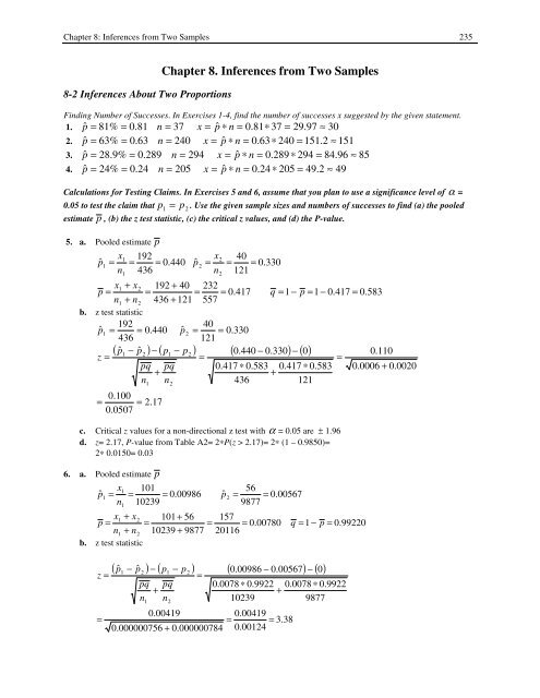
Chapter 8: Inferences from Two Samples 2358-2 Inferences About Two ProportionsChapter 8. Inferences from Two SamplesFinding Number of Successes. In Exercises 1-4, find the number of successes x suggested by the given statement.1. p ˆ = 81% = 0.81 n = 37 x = pˆ∗ n = 0.81∗37 = 29.97 ≈ 302. p ˆ = 63% = 0.63 n = 240 x = pˆ∗ n = 0.63∗240 = 151.2 ≈ 151p ˆ = 28.9% = 0.289 n = 294 x = pˆ∗ n = 0.289 ∗ 294 = 84.96 ≈4. p ˆ = 24% = 0.24 n = 205 x = pˆ∗ n = 0.24 ∗ 205 = 49.2 ≈ 493. 85Calculations for Testing Claims. In Exercises 5 and 6, assume that you plan to use a significance level of α =0.05 to test the claim that p1= p2. Use the given sample sizes and numbers of successes to find (a) the pooledestimate p , (b) the z test statistic, (c) the critical z values, and (d) the P-value.5. a. Pooled estimate px1192pˆ1= = = 0.440n 4361pˆ2x=n22=40121= 0.330x1+ x2192 + 40 232p = = = = 0.417 q = 1 − p = 1 − 0.417 = 0.583n1+ n2436 + 121 557b. z test statistic19240pˆˆ1= = 0.440 p2= = 0.330436121( pˆˆ1− p2) − ( p1− p2) ( 0.440 − 0.330) − ( 0)0.110z ===pq pq 0.417 ∗ 0.583 0.417 ∗ 0.583 0.0006 + 0.0020++n n436 121=0.1000.05071= 2.172c. Critical z values for a non-directional z test with α = 0.05 are ± 1.96d. z= 2.17, P-value from Table A2= 2∗P(z > 2.17)= 2∗ (1 – 0.9850)=2∗ 0.0150= 0.036. a. Pooled estimate px1101pˆ1= = = 0.00986n110239x1+ x2101+56p = ==n1+ n210239 + 9877b. z test statisticz ==pˆ2=15720116569877= 0.00567= 0.00780( pˆ− pˆ) − ( p − p ) ( 0.00986 − 0.00567) − ( 0)12pqn1+1pqn22=0.004190.00419= = 3.380.000000756 + 0.000000784 0.00124q = 1−p = 0.992200.0078 ∗ 0.9922 0.0078 ∗ 0.9922+102399877

236 Chapter 8: Inferences from Two Samplesc. Critical z values for a non-directional z test with α = 0.05 are ± 1.96d. z= 3.38, P-value from Table A2= 2∗P(z > 3.38)= 2∗ (1 – 0.9996)=2∗ 0.0004= 0.00087. Exercise and Heart DiseaseTo find the 0.90 or 90% confidence interval, the critical values of z are ±1.645pˆ1pˆ2x=n11x=n22101= = 0.0098610239=569877= 0.00567= 1−pˆpˆˆ1− p2= 0.00986 − 0.00567 = 0.00419CI = pˆ− pˆ− E < p − p < pˆ− pˆ= 1.645CICICI90%E = z90%90%90%α / 2===qˆqˆ11= 1−pˆ( ) ( ) ( )1pˆˆ1qn112pˆˆ2q2+n2= 1.6450.000000953 + 0.000000571 = 1.64511= 1−0.00986 = 0.99014= 1−0.00567 = 0.994330.00986 ∗ 0.99014 0.00567 ∗ 0.99433+1023998770.000001524 = 1.645∗0.00123 = 0.00203( 0.00986 − 0.00567) − 0.00203 < ( p1− p2) < ( 0.00986 − 0.00567)0.00419 − 0.00202 < ( p1− p2) < 0.00419 + 0.002020.00216 < ( p − p ) < 0. 00622112212+ E+ 0.00203The confidence interval does not contain zero. Therefore, it appears that physical activity corresponds to a lowerrate of coronary artery disease.8. Exercise and Heart Disease, from Exercise 7Assume group 1 is the low activity group and group 2 is the high activity groupWill conduct a directional z test to test the hypotheses:H0: p1− p2= 0 H1: p1− p2> 0With α = 0.05 and a directional test where a positive z value supports the research (H 1 ) hypothesis, the criticalvalue (CV) of z is +1.645pˆˆ1= 0.00986 q1= 0.99014pˆˆ1− p2= 0.00419x1+ x2101+56pˆ= ==n + n 10239 + 9877σ=zp1− p2p1− p21=2pq ˆ ˆ+n( pˆ− pˆ)157201160.000000756 + 0.000000784 ==11σpq ˆ ˆ=n22− µp1− p2p1− p2pˆ2= 0.00567= 0.007800.00419 − 0== 3.380.00124qˆ0.00780 ∗ 0.99220 0.00780 ∗ 0.99220+1023998770.00000154 = 0.001242= 0.99433qˆ= 1−pˆ= 1−0.00780 = 0.99220The observed z statistic is in the region of rejection of the null since it is higher than +1.645. The P-value forthis test statistic is, from Table A2= 2∗P(z > 3.38)= 2∗ (1 – 0.9996)=2∗ 0.0004= 0.0008. Both of these, the z statistic and P-value (consistently) indicate the Null should berejected, supporting the inference that the proportion of women in the low activity group having heart disease issignificantly higher than heart disease in the high activity group.

Chapter 8: Inferences from Two Samples 2379. Effectiveness of Smoking BansH : p = p H : p ≠ p05627pˆˆ1= = 0.0664 p2= = 0.0384843703x1+ x256 + 27p = = = 0.0537 q = 1 − p = 0.9463n + n 843 + 7031122112z ==( pˆ− pˆ) − ( p − p ) ( 0.0664 − 0.0384) − ( 0)12pqn1+1pqn0.0280 0.0280= = 2.430.0001326 0.011522=0.0537 ∗ 0.9463 0.0537 ∗ 0.9463+843703=0.02800.0000603 + 0.0000723When α is set at 0.05, there is a significant difference since the observed z of 2.43 is greater than +1.96 and theP-value is 2∗ (1 – 0.9925) = 2∗ 0.0075= 0.0150, which is lower than α = 0.05.When α is set at 0.01, there is not a significant difference since the observed z of 2.43 is not greater than+2.575. The P-value is the same at 0.0150 and it is higher than α of 0.01, indicating lack of statisticalsignificance at this level of α .10. Effectiveness of the Salk VaccineAssume group 1 is the vaccinated group and group 2 is the non-vaccinated groupWill conduct a directional z test to test the hypotheses:H0: p1− p2= 0 H1: p1− p2< 0With α = 0.01 and a directional test where a positive z value supports the research (H 1 ) hypothesis, the criticalvalue (CV) of z is -2.326A value lower than -2.326 would indicate a significant directional differenceH0: p: p33115pˆˆ1= = 0.000164 p2= = 0.000571200745201229x1+ x233 + 115 148p = == = 0.000368n + n 200745 + 201229 40197411=2p2H11

238 Chapter 8: Inferences from Two Samples11. Color Blindness in Men and Womena. Assume group 1 is male and group 2 is femaleWill conduct a directional z test to test the hypotheses:H0: p1− p2= 0 H1: p1− p2> 0With α = 0.01 and a directional test where a positive z value supports the research (H 1 ) hypothesis, thecritical value (CV) of z is +2.326A value higher than +2.326 would indicate a significant directional difference456pˆˆ1= = 0.09000 p2=5002100= 0.00286x1+ x2 45 + 6 51p = ==n + n 500 + 2100 2600= 0.0196 q = 1 − p = 0.980412z==( pˆ− pˆ) − ( p − p ) ( 0.09000 − 0.00286 ) − ( 0)12pqn1+0.00003841pqn20.087142=+ 0.000009150.0196 ∗ 0.9804500=0.087140.00004760.0196 ∗ 0.9804+2100=0.087140.00690= 12.64With α = 0. 01, since the observed z statistic (12.64) is higher than the critical value of +2.326, the malegroup has a significantly higher rate of red/green color blindness than women. The P-value (determinedusing Excel) is ~ 0, clearly lower than 0.01.b. Find CI 98%CI = pˆ− pˆ− E < p − p < pˆ− pˆ+ ECICI98%E = z= 2.32698%98%α / 2==( ) ( ) ( )1pˆ1qˆn112pˆ2qˆ2+n= 2.3260.000163800 + 0.00000136 = 2.3260.0900 ∗ 0.9100 0.00286 ∗ 0.99714+50021000.00016516 = 2.326 ∗ 0.0129 = 0.0299( 0.09000 − 0.00286) − 0.0299 < ( p1− p2) < ( 0.09000 − 0.00286)0.0572 < ( p − p ) < 0. 11701221212+ 0.0299The confidence interval does not contain zero, thus there seems to be a significant difference between menand women with respect to red/green color blindness.c. We need a large sample size for women so that the requirements of:≥ 5 and ≥ 5 are both satisfied, so use of the normal approximation is justifiednpnq12. Seat Belts and Hospital TimeAssume group 1 is children not wearing seat belts and group 2 is children wearing seat beltsWill conduct a directional z test to test the hypotheses:H0: p1− p2= 0 H1: p1− p2> 0With α = 0.05 and a directional test where a positive z value supports the research (H 1 ) hypothesis, the criticalvalue (CV) of z is +1.645A value higher than +1.645 would indicate a significant directional difference

Chapter 8: Inferences from Two Samples 2395016pˆˆ1= = 0.1724 p2= = 0.1301290123x1+ x250 + 16 66p = = = = 0.1598n + n 290 + 123 41312q= 1−p = 0.8402z =( pˆ− pˆ) − ( p − p ) ( 0.1724 − 0.1301) − ( 0)12pqn1+1pqn22=0.1598 ∗ 0.8402 0.1598 ∗ 0.8402+1232900.04230.0423 0.0423=== = 1.070.001092 + 0.000463 0.001555 0.0394At α = 0. 05 with a directional test, since the observed z statistic is not higher than +1.645, there is not asignificantly higher incidence of severe injury for children not wearing seat belts compared with children whouse seat belts. The P-value for this test statistic is, from Table A2= P(z > 1.07)= (1 – 0.8577) =0.1423.13. Drinking and CrimeAssume group 1 is drinkers convicted of arson and group 2 is drinkers convicted of fraudWill conduct a directional z test to test the hypotheses:H0: p1− p2= 0 H1: p1− p2> 0With α = 0.01 and a directional test where a positive z value supports the research (H 1 ) hypothesis, the criticalvalue (CV) of z is +2.326A value higher than +2.326 would indicate a significant directional difference5063pˆˆ1= = 0.5376 p2= = 0.304393207x1+ x250 + 63 113p = = = = 0.3767 q = 1−p = 0.6233n + n 93 + 207 300z =1( pˆ− pˆ) − ( p − p ) ( 0.5376 − 0.3043) − ( 0)122pqn1+1pqn22=0.3767 ∗ 0.6233 0.3767 ∗ 0.6233+932070.23330.2333 0.2333=== = 3.860.002525 + 0.001134 0.003659 0.0605Since the observed z statistic is higher than the critical value, we conclude the proportion of drinkers whocommitted arson was significantly higher than the proportion of drinkers who committed fraud. The differencetype of crime committed seems to be related to drinking. Arson would seem to be more of a crime of “passion”or violence than fraud so it would seem that drinking might make a criminal commit more such crimes.14. Testing Laboratory GlovesAssume group 1 is vinyl gloves and group 2 is latex glovesWill conduct a directional z test to test the hypotheses:H0: p1− p2= 0 H1: p1− p2> 0With α = 0.005 and a directional test where a positive z value supports the research (H 1 ) hypothesis, the criticalvalue (CV) of z is +2.575A value higher than +2.575 would indicate a significant directional difference

240 Chapter 8: Inferences from Two Samplesx11151pˆ1= =240x1+ x2p =n + nz == n1= 240 ∗ 0.63 = 151,170.6292 pˆ2= = 0.0708240151+17 168= = = 0.3500240 + 240 480q = 1−p = 0.6500( pˆ− pˆ) − ( p − p ) ( 0.6292 − 0.0708) − ( 0)1∗ p122pqn1+1pqn22=x2= n2∗ p= 240 ∗ 0.07 = 170.35 ∗ 0.65 0.35 ∗ 0.65+240 24020.5584 0.5584 0.5584== = = 12.810.00095 + 0.00095 0.0019 0.0436Since the observed z statistic is higher than the critical value, we conclude the proportion of vinyl gloves thatleak is significantly higher than the proportion of latex gloves that leak.15. Written Survey and Computer SurveyAssume group 1 takes the written survey and group 2 takes a computer surveyWill conduct a non-directional z test to test the hypotheses:H0: p1− p2= 0 H1: p1− p2≠ 0Let’s set α = 0.01 and a non-directional test, the critical values (CV) of z are ±2.575A value lower than -2.575 or higher than +2.575 would indicate a significant difference in admitting theycarried a guna. z testx = n ∗ p = 850 ∗ 0.079 = 67, x = n ∗ p = 850 ∗ 0.124 = 1051167pˆ1= =850x1+ x2p =n + nz =11050.0788 pˆ2= = 0.123585067 + 105 172= = = 0.1012850 + 850 1700q = 1−p = 0.8988( pˆ− pˆ) − ( p − p ) ( 0.0788 − 0.1235) − ( 0)1122pqn1+1pqn22=220.1012 ∗ 0.8988 0.1012 ∗ 0.8988+850850− 0.0447 − 0.0447 − 0.0447=== = −3.060.000107 + 0.000107 0.000214 0.0146Since the observed z statistic is lower than the CV of -2.575, there is a significant difference in theproportion of respondents who admit to carrying a gun when taking a written rather than a computersurvey. The P-value would be 2 ∗ (1 – P(z < 3.06)) =2 ∗ (1 – 0.9989)= 2 ∗ 0.0011= 0.0022.b. Find CI 99%CI = ( pˆ− pˆ) − E < ( p − p ) < ( pˆ− pˆ)CICI99%E = z= 2.57599%99%α / 2=1pˆˆ1qn1122= 2.5750.0000854 + 0.0001274 = 2.575( 0.0788 − 0.1235) − 0.0376 < ( p1− p2) < ( 0.0788 − 0.1235)0.0823 < ( p − p ) < −0.0071= −pˆˆ2q+n12122122+ E0.0788∗0.9212 0.1235∗0.8765+8508500.0002128 = 2.575∗0.0146 = 0.0376+ 0.0376

Chapter 8: Inferences from Two Samples 243Let’s set α = 0.05 and a non-directional test, the critical values (CV) of z are ±1.96A value lower than -1.96 or higher than +1.96 would indicate a significant difference in treatment results6760pˆ0.9178 ˆ1= =p2= = 0.72297383xp =nz =1167=7360=83127156= 0.8141q = 1−p = 0.1859( pˆ− pˆ) − ( p − p ) ( 0.9178 − 0.7229) − ( 0)1+ x+ n222pqn1+++1pqn22=0.8141∗0.1859 0.8141∗0.1859+73830.19490.1949 0.1949=== = 3.1220.002073 + 0.001823 0.003896 0.06242Withα= 0. 05 , for a non-directional test, since the observed z statistic is higher than + 1.96, there is asignificant difference in treatment success rate. The P-value would be2 ∗ (1 – P( z < 3.12)) = 2 ∗ (1 – 0.9991)= 2 ∗ 0.0009= 0.0018. It would appear that the success rate fromsurgery is higher than the use of a splint.20. Health SurveyAssume group 1 is the male group and group 2 is the female group and the dependent variable is proportion inthe group over 30 years of ageWill conduct a non-directional z test to test the hypotheses:H0: p1− p2= 0 H1: p1− p2≠ 0Let’s set α = 0.05 and a non-directional test, the critical values (CV) of z are ±1.96A value lower than -1.96 or higher than +1.96 would indicate a significant difference in treatment results2322pˆˆ1= = 0.575 p2= = 0.5504040x1+ x223 + 22 45p = = = = 0.5625 q = 1−p = 0.4375n + n 40 + 40 80z =1( pˆ− pˆ) − ( p − p ) ( 0.575 − 0.550) − ( 0)122pqn1+1pqn22=0.5625 ∗ 0.4375 0.5625 ∗ 0.4375+40400.0250.025 0.025=== = 0.2250.006152 + 0.006152 0.012320 0.1109Withα = 0. 05 , for a non-directional test, since the observed z statistic is not lower than -1.96 or higher than +1.96, there is a not significant difference in proportion of males and females above 30 year of age. The P-valuewould be 2 ∗ (1 – P(z < 0.23)) = 2 ∗ (1 – 0.5910)= 2 ∗ 0.4090= 0.8180. Using Excel and a z value of 0.225, theP-value is 0.8220.

244 Chapter 8: Inferences from Two Samples*21. Interpreting Overlap of Confidence Intervalsa. Find CI 95% for the difference in the two proportions11288pˆˆ1= = 0.5600 p2= = 0.4400200200CI = pˆ− pˆ− E < p − p < pˆ− pˆCICI95%E = z= 1.9695%95%α / 2==( ) ( ) ( )1pˆˆ1qn112pˆˆ2q2+n= 1.960.001232 + 0.001232 = 1.960.5600 ∗ 0.4400 0.4400 ∗ 0.5600+2002000.002464 = 1.96 ∗ 0.0496 = 0.0973( 0.5600 − 0.4400) − 0.0973 < ( p1− p2) < ( 0.5600 − 0.4400)0.0227 < ( p − p ) < 0.21731221212+ E+ 0.0973The confidence interval does not contain zero. Therefore, there appears to be a significant differencebetween the two proportions.b. Individual single group confidence intervalsCI95%for pˆpq ˆ ˆ 0.5600 ∗ 0.4400E = zα/ 2= 1.96= 1.96 0.001232 = 1.96 ∗ 0.0351 = 0.0688n200CI for pˆ= 0.5600 − 0.0688 < p < 0.5600 + 0.0688 = 0.4912 < p < 0.628895%11= pˆ− E

Chapter 8: Inferences from Two Samples 245d. In order to test the Null hypothesis of H0: p1− p2= 0 , either the z test can be used or the confidenceinterval of the difference in the proportions can be used, with consistent results. However, comparing theindividual group proportion confidence intervals and basing the decision on looking for overlap or lack ofoverlap of the confidence intervals is the least effective option and it should not be used.*22. Equivalence of Hypothesis Test and Confidence IntervalAssume group 1 is the first sample and group 2 is the second sampleWill conduct a non-directional z test to test the hypotheses:H0: p1− p2= 0 H1: p1− p2≠ 0Let’s set α = 0.05 and a non-directional test, the critical values (CV) of z are ±1.96A value lower than -1.96 or higher than +1.96 would indicate a significant difference in the two proportions101404pˆˆ1= = 0.5000 p2= = 0.7020202000x1+ x210 + 1404 1414p = = = = 0.7000 q = 1−p = 0.3000n + n 20 + 2000 2020z =1( pˆ− pˆ) − ( p − p ) ( 0.5000 − 0.7020) − ( 0)122pqn1+1pqn22=0.7000 ∗ 0.3000 0.7000 ∗ 0.3000+202000− 0.2020 − 0.2020 − 0.2020=== = −1.9620.010500 + 0.000105 0.010605 0.1030Withα= 0. 05 , for a non-directional test, since the observed z statistic is lower than-1.96, there is a significant difference in the two proportions. The P-value would be2 ∗ (1 – P(z < 1.96)) = 2 ∗ (1 – 0.9750)= 2 ∗ 0.0250= 0.0500. The P-value forz= -1.962 (from Excel) is 0.0498, less than 0.05. Thus, H0: p1− p2= 0 is rejected,supporting H p − p 0 .0:1 2≠Finding CI 95%pˆ= 0.50001CICICI95%E = z= 1.9695%95%=α / 2=pˆ( pˆ− pˆ) − E < ( p − p ) < ( pˆ− pˆ)1pˆˆ1qn1122= 0.7020= 1.960.012500 + 0.000105 = 1.960.5000 ∗ 0.5000 0.7020 ∗ 0.2980+2020000.012605 = 1.96 ∗ 0.1123 = 0.2200( 0.5000 − 0.7020) − 0.2200 < ( p1− p2) < ( 0.5000 − 0.7020)0.422 < ( p − p ) < 0. 018= −pˆˆ2q+n12221212+ E+ 0.2200The confidence interval contains zero. Therefore, there appears to not be a significant difference between thetwo proportions.For this example, the test statistic and confidence interval lead to different conclusions. While this is a possibleoutcome, the two approaches usually lead to the same decision about the rejection of the Null hypothesis.*23. Testing for Constant DifferenceWill conduct a non-directional z test to test the hypotheses:H0: p1− p2= 0.1 H1: p1− p2≠ 0.1Let’s set α = 0.05 and a non-directional test, the critical values (CV) of z are ±1.96A value lower than -1.96 or higher than +1.96 would indicate a significant difference in the two proportions

246 Chapter 8: Inferences from Two Samplesx1111729pˆˆ1= = 0.1594 p2= = 0.0400734725x1+ x2117 + 29 146p = = = = 0.1001n + n 734 + 725 1459z == n1∗ p( pˆ− pˆ) − c ( 0.1594 − 0.0400)1pˆˆ1qn1112= 734 ∗ 0.16 = 117,2pˆˆ2q2+n2=x2= n2∗ p= 725 ∗ 0.04 = 29− 0.100.1594 ∗ 0.8406 0.0400 ∗ 0.9600+7347252q = 1−p = 0.89990.01940.0194 0.0194=== = 1.260.000183 + 0.000053 0.000236 0.0154Withα = 0. 05 , for a non-directional test, since the observed z statistic is not lower than -1.96 or higher than +1.96, there is not a significant difference in the two proportions. The P-value would be 2 ∗ (1 – P(z > 1.26)) = 2∗ (1 – 0.8962)= 2 ∗ 0.1038= 0.2076. Thus, there is no evidence to indicate the headache rate for Viagra users is10% different than that of the headache rate for men given a placebo.8-3 Inferences About Two Means: Independent SamplesIndependent Samples and Matched Pairs. In Exercises 1-4, determine whether the samples are independent orconsist of matched pairs.1. Independent since groups are comprised of different subjects.2. Matched pairs since the same subjects are measured twice.3. Matched pairs since the data are matched on both their estimate and the physician’s scale.4. Independent since groups are comprised of different cans of soda.In Exercises 5-24, assume that the two samples are independent simple random samples from normallydistributed populations. Do not assume that the population standard deviations are equal.Note: In the 5-24 Exercises below, degrees of freedom (df) are computed based on the smaller sample size – 1.This approach is used when the assumption that the samples are drawn from normal distributions is notmade. Many other examples of this test comparing two means use another approach to finding the degrees offreedom as df= n 1 + n 2 – 2 whether or not this normality assumption is made. Use of the smaller sample size –1 for df is considered a conservative approach.5. Hypothesis Test for Effect of Marijuana Use on College StudentsConduct independent t test

Chapter 8: Inferences from Two Samples 247Hnnx1210α = 0.01,df= nt =: µ= 64, x= 65, x− x= µ= 533 . , s= 513 . , s= 53.3 − 513 . = 2.000( x − x ) − ( µ − µ ) ( 533 . -513. )11212222s1n11s+nH: µ= 3.6= 4.5−1= 63,t122211221> µ=α22= + 2.390 (using df =3.6642− 0=24.5+6560, from Table A - 3)2.00 2.00= = 2.790.5140 0.7170Since the test statistic (2.79) is greater than the t critical value (+2.390), we reject the null hypothesis andconclude that the population of heavy marijuana users have a lower mean mental ability score than the lightusers. P-value (from Excel)= 0.003, which is less than 0.01.6. Confidence Interval for Effect of Marijuana Use on College StudentsFind CI. 98% for Example 5α = 0.02,dfE = tCI98%α2=sn211= 2.000= 0.286= n −1= 63,ts+n2221= 2.3903.6644.5+65= 2.390( x1− x2) − E < ( µ1− µ2) < ( x1− x2)−1714. < ( µ1− µ2) < 2.000 + .< ( µ − µ ) < 3.71412α2= + 2.390 (using df =221714+ E60, from Table A - 3)0.5140 = 2.390 ∗ 0.7170 = 1714 .The confidence interval does not include zero, therefore, we conclude that the two population means are notequal.7. Confidence Interval for Magnet Treatment of Pain, Find CI 90%nnx121= 20, x= 20, xα = 010 . ,dfE = tCI− x90%2α2=12= 0.49 − 0.44 = 0.050sn21( x1− x2) − E < ( µ1− µ2) < ( x1− x2). − 0.656 < ( µ1− µ2) < 0.050 + .0.606 < ( µ − µ ) < 0.706= 0 050= −= 0.49, s1= 0.44, s= n1s+n222= 0.96= 140 .−1= 20 −1= 19,t= 1729 .11220.96202α2140 .+20= ± 1729 . (from Table A - 3)2= 1729 .+ E0 65601441 . = 1729 . ∗ 0.3796 = 0.656The confidence interval contains zero. Therefore we conclude that there is no difference between the two meansand that the magnetic treatment is not effective in reducing pain.

248 Chapter 8: Inferences from Two Samples8. Hypothesis Test for Magnet Treatment of Pain, Conduct independent t test for data in Exercise 7H0t =df: µ( x − x ) − ( µ − µ ) ( 0.490 - 0.440)11= µ22sn211= 20 −1=1s+n222H1: µ21=> µ20.9620− 0=21.40+2019, t = + 1729 . (from Table A − 3)20.050=0.14410.0500.3796= 0.132Since the test statistic (0.132) is less than the critical t (+1.729), we do not reject the null hypothesis and weconclude that there is no difference between the means of the two samples. The magnets do not appear to beeffective in reducing back pain. If the sample sizes were larger, the magnets may appear to be effective becausein the above example, n

Chapter 8: Inferences from Two Samples 24911. Confidence Interval for Effects of Alcohol, Find CI 95%nnx121= 22, x= 22, xα = 0.05,dfE = tCI− x95%2α2=12= 4.20 −171. = 2.49sn21= 1463 .= 4.20, s1= 171 . , s1s+n222= 2.20= 0.72= 2.0802.20220.72+22= 2.080 (from Table A - 3)= 2.0800.2436 = 2.080 ∗ 0.4935 = 1027 .( x1− x2) − E < ( µ1− µ2) < ( x1− x2) + E = 2.490 −1027. < ( µ1− µ2)< ( µ − µ ) < 3.517112= n −1= 22 −1= 21,t22α22< 2.490 + 1027 .The confidence interval does not include zero, therefore, we conclude that there is a significant differencebetween the two population means, and that significantly more errors are made by those who are treated withalcohol.12. Hypothesis Test for Effects of Alcohol, Conduct independent t test for data in Exercise 11H0t =: µ= µ( x − x ) − ( µ − µ ) ( 4.20-171. )1122s1nα = 0.05, df211s+n222H1: µ21== 22 −1=≠ µ22.20222− 020.72+222.49= = 5.040.493621, t = ± 2.080 (from Table A − 3)Since the test statistic (5.04) is higher than +2.080, we reject the null hypothesis and we conclude that there is adifference between the errors made by those who are treated with alcohol compared with those not treated withalcohol.13. Poplar Trees, Find CI 95%nnx121= 5, xE = t= 5, x− x95%2α2=12= 0.127= 0.184 −1.334= −1.150α = 0.05,df = nCI= −= 0.184, ssn211s+n1222−1= 5 −1= 4,t= 2.776= 0.8590.1275= ± 2.776 (from Table A - 3)0.859+5= 2.7760.1508 = 2.776 ∗ 0.3883 = 1.078( x1− x2) − E < ( µ1− µ2) < ( x1− x2) + E = −1.150−1.078< ( µ1− µ2)2.228 < ( µ − µ ) < −0.07211= 1.334, s22α222< −1.150+ 1.078The confidence interval does not include zero, therefore, we conclude that there is a significant differencebetween the weights of the two groups of poplar trees given different treatments.

250 Chapter 8: Inferences from Two Samples14. Poplar Trees, Conduct independent t test for data from Exercise 13H0t =: µ( x − x ) − ( µ − µ ) ( 0.184 -1.334)11= µ22sn21α = 0.05, df11s+n222H1: µ2= 5 −1=1=≠ µ20.12952− 00.859+5-1.1500.38834, t = ± 2.776 (from Table A − 3)2== −2.962The test statistic (-2.962) is lower than -2.776. Therefore, we reject the null hypothesis and conclude that thereis a significant difference between the weights of the two groups of poplar trees given different treatments.15. Petal Lengths of Irises, Conduct independent t testn = 50,xn12H0t =: µ= 146 . , s= 4.26, s= 017 .= 0.47: µ50 −1= 49, t = ± 2.009 (from Table A − 3)( x − x ) − ( µ − µ ) ( 146 . -4.26)111= 50,x22= µα = 0.05, df =2sn2111s+n222H11221=≠ µ2017 .502− 00.47+502=− 2.8 -2.8= = −39.600.004996 0.0707The test statistic (-39.6) is lower than -2.009. Thus, we reject the null hypothesis and conclude that there is asignificant difference between the mean petal length of irises in the two populations.16. Petal Lengths of Irises, Find CI 95% for data in Exercise 15α = 0.05, df =E = tCI95%α2== −sn211s+n50 −1= 49, t = ± 2.009 (from Table A − 3)222= 2.009017 .500.47+50= 2.009 ∗ 0.0707 = 01420 .( x1− x2) − E < ( µ1− µ2) < ( x1− x2) + E = −2.8 − 01420 . < ( µ1− µ2)2.942 < ( µ − µ ) < −2.6581222< −2.8 + 01420 .The confidence interval does not include zero, therefore, we conclude that there is a significant differencebetween the mean petal length of irises in the two populations.17. BMI of Men and Women, Conduct independent t testn = 40,xnx121α = 0.05,dfH0t =− x2: µ= 25.998, s= 25.740, s= 25.998 − 25.740 = 0.258: µ= 3.431= 6166 .( x − x ) − ( µ − µ ) ( 25.998-25.740)111= 40,x22= µ2sn21111s+n222H121= n −1= 40 −1= 39,t21=≠ µ23.43140α22= ± 2.024 (from Table A - 3)− 0=26166 .+400.258 0.258= = 0.2311.2448 1116 .The test statistic is not greater than +2.024. Therefore, we do not reject the null hypothesis and we conclude thatthere is not enough evidence to support the claim that the BMI of men and women are not equal.

Chapter 8: Inferences from Two Samples 25118. BMI of Men and Women, Find CI 95% for data in Exercise 17α = 0.05,dfE = tCI95%α2=sn211( x1− x2) − E < ( µ1− µ2) < ( x1− x2) + E = 0.258 − 2.259 < ( µ1− µ2). < ( µ − µ ) < 2.517= −2 001= n −1= 40 −1= 39,t1s+n222= 2.024123.431402α2= ± 2.024 (from Table A - 3)6166 .+402= 2.024 ∗1.116= 2.259< 0.258 + 2.259The confidence interval contains zero, therefore we conclude that there is no significant difference betweenBMI of men and women.19. Head Circumferences, Conduct independent t testn = 50,xnx121α = 0.05,dfH0t =− x2: µ= 41098 . , s= 40.048, s= 41.098 − 40.048 = 1.050: µ= 1498 .= 1640 .( x − x ) − ( µ − µ ) ( 41098 . -40.048)111= 50,x22= µ2sn21111s+n222H121= n −1= 50 −1= 49,t21=≠ µ21498 .50α22= ± 2.009 (from Table A - 3)− 0=21640 .+501.050 1050 .= = 3.3430.09867 0.3141The test statistic (3.343) is higher than +2.009. Thus, we reject the null hypothesis and conclude that there isenough evidence to support the claim that the head circumference of males and females is significantlydifferent.20. Head Circumferences, Find CI 95% for data in Exercise 19α = 0.05,dfE = tCI95%α2=sn211( x1− x2) − E < ( µ1− µ2) < ( x1− x2) + E = 1050 . − 0.631 < ( µ1− µ2)< ( µ − µ ) < 1.681= 0.419= n −1= 50 −1= 49,t1s+n222= 2.009121498 .502α2= ± 2.009 (from Table A - 3)1640 .+502= 2.009 ∗ 0.3141 = 0.631< 1050 . + 0.631The confidence interval does not include zero, therefore, we conclude that there is a significant differencebetween the mean head circumference of male and female two month old babies.

252 Chapter 8: Inferences from Two Samples21. Seat Belts and Hospital Time, Conduct independent t testnnx121α = 0.01,dfH0t ==− x: µ290, x20.83, s= 1.39 − 0.83 = 0.56−1= 123 −1= 122,t: µ= 3.06= 177 .( x − x ) − ( µ − µ ) ( 139 . -0.83)11= µ21= 123, x2sn221= n1= 139 . , s=, H211s+n2221212> µ2=23.06290α2− 02177 .+123= + 2.364 (use df== 100 from Table A - 3)0.56 0.56= = 2.3300.05776 0.2403The test statistic (2.33) is not higher than the critical value of 2.364. Thus, we do not reject the null hypothesisand we conclude that there is not enough evidence to support the claim that seat belt use leads to a lower stay inhospital.22. Seat Belts and Hospital Time, Find CI 95% for data in Exercise 21α = 0.05,dfE = tCI95%α2=sn211= 0.083= n −1= 123 −1= 122,t1s+n222= 1984 .23.062902177 .+123= ± 1984 . (use df= 1984 . ∗ 0.2403 = 0.477= 100, from Table A - 3)( x1− x2) − E < ( µ1− µ2) < ( x1− x2) + E = 0.56 − 0.477 < ( µ1− µ2)< ( µ − µ ) < 1.03712α2< 0.56 + 0.477The confidence interval does not include zero, therefore, we conclude that there is a significant differencebetween the hospital stay of children that wear seat belts compared to children that do not wear seat belts.23. Effects of Cocaine on Children, Conduct independent t testnnx121α = 0.05,dfH0t == 190, x− x2: µ= 7.3, s= 8.2, s= 3.0= 3.0= 7.3 − 8.2 = −0.09−1= 186 −1= 185,t( x − x ) − ( µ − µ ) ( 7.3-8.2)11= µ21= 186, x2sn2211= n21s+n222H112α2: µ1< µ22=− 0=2 23.0 3.0+190 186= −1653 . (use df= 200 from Table A - 3)− 0.9 -0.9= = −2.9080.09576 0.3094The test statistic (-2.908) is lower than the critical value of -1.653. Therefore, we reject the null hypothesis andconclude that there is enough evidence to support the claim that prenatal cocaine exposure is associated withlower scores of four-year old children on the test of object assembly.

Chapter 8: Inferences from Two Samples 25324. Birth Weight and IQ, Conduct independent t testnnx121α = 0.05,dfH0t ===− x: µ258, x220, x2= 95.5, s= 104.9, s= 95.5 −104.9= −9.40−1= 220 −1= 219,t: µ= 16.0= 141 .( x − x ) − ( µ − µ ) ( 95.5-104.9)11=µ212sn2112= n21s+n222H11221=≠µ216.02582α2− 0=2141 .+220= ± 1.972 (use df=− 9.4 -9.4= = −6.8271.896 1377 .200 from Table A - 3)The test statistic (-6.827) is lower than -1.972. Therefore, we reject the null hypothesis and conclude that thereis enough evidence to support the claim that there is a difference in the mean IQ of low birth weight babiescompared to normal babies.In Exercises 25-28, assume that the two samples are independent simple random samples selected from normallydistributed populations. Also assume that the population standard deviations are equal (σ 1 = σ 2 ). So that thestandard error of the differences between means is obtained by pooling the sample variances.25. Hypothesis Test with Pooling, t test from Exercise 5 conducted with normality assumptionHnnx121: µ= 64, x= 65, xα = 0.01,dfs2p0t =− x2= 53.3, s= 513 . , s: µ= 3.6= 4.5= 533 . − 513 . = 2.0002( n1−1) s1+ ( n2−1)( n1−1) + ( n2−1)( x − x ) − 0=11sn= µ2p11222s+n2p21H112= n + n=21− 2 = 64 + 65 − 2 = 127,ts> µ22=2.0=16.63 16.63+64 652α22( 64 −1) ∗ 3.6 + ( 65 −1)( 64 −1) + ( 65 −1)= + 2.364(using df∗ 4.52.0 2.0= = 2.7850.5157 0.7182= 100, from Table A - 3)2112.48= = 16.63127The test statistic (2.785) is higher than the critical value of +2.364. We reject the null hypothesis and concludethat there is enough evidence to support the claim that heavy marijuana users have a lower mean than light usersjust as we did in Exercise 5. Results are not affected by this additional assumption. However, the critical valuein this case is lower than the critical value used in Exercise 5 (2.390).

254 Chapter 8: Inferences from Two Samples26. Confidence Interval with Pooling, Confidence interval from Exercise 6 with normality assumptionnnx1212p= 64, xE = t= 65, x− x=98%2= 533 . − 513 . = 2.0002( n1−1) s1+ ( n2−1)( n −1) + ( n −1)α2=1122( 64 −1) ∗3.6+ ( 65 −1)( 64 −1) + ( 65 −1)( x1− x2) − E < ( µ1− µ2) < ( x1− x2) + E = 2.0 −1.697< ( µ1− µ2)< ( µ − µ ) < 3.697= 0.303= 53.3, s2p1= 513 . , sα = 0.02,df = nsCIsns+n12p2= 3.6= 4.5− 2 = 64 + 65 − 2 = 127,t= 2.3641212+ n22s22=16.636416.63+65α2= ± 2.364 (using df∗ 4.5= 2.364 ∗ 0.718 = 1.6972== 100, from Table A - 3)2112.48= 16.63127< 2.0 + 1.697The confidence interval does not include zero, therefore, we conclude that heavy marijuana users have a meanmental ability that is significantly different than that of light users. This is the same outcome as found inExercise 6. However, notice that the confidence interval is narrower when the normality assumption is made.The CI 98% found in Exercise 6 was 0.286 to 3.714.27. Confidence Interval with Pooling, Confidence interval from Exercise 7 with normality assumptionnnx121= 20, x= 20, xα = 010 . , dfs2pE = tCI− x=90%2= 0.49, s= 0.44, s= 0.49 − 0.44 = 0.0502( n1−1) s1+ ( n2−1)( n −1) + ( n −1)α2== −112sn2p11s+n2p2= 0.96= 140 .= 1686 .− 2 = 20 + 20 − 2 = 38,t2( 20 −1) ∗ 0.96 + ( 20 −1)( 20 −1) + ( 20 −1)0.9216+200.921620= 1.686= ± 1.686 (from Table A - 3)∗1.40.14408 = 1.686 ∗ 0.3796 = 0.640( x1− x2) − E < ( µ1− µ2) < ( x1− x2) + E = 0.05 − 0.64 < ( µ1− µ2)0.59 < ( µ − µ ) < 0.691212= n + n22s22=α2254.7504= = 1.440838< 0.05 + 0.64The confidence interval contains zero. Therefore we conclude that there is no difference between the two meansand that the magnetic treatment is not effective in reducing pain. This is the same result that was obtainedearlier. However, in this case the confidence interval is narrower (in Exercise 7, CI 90% was -0.606 to 0.706).

Chapter 8: Inferences from Two Samples 25528. Hypothesis Test with Pooling, t test from Exercise 8 conducted with normality assumptionnnx121= 20, x= 20, xα = 0.05,dfHs2p0t =− x2: µ= 0.49, s= 0.44, s= 0.96= 0.49 − 0.44 = 0.050: µ2( n1−1) s1+ ( n2−1)( n1−1) + ( n2−1)( x − x ) − 0 0.05=11sn2p112= µ22s+n2p21H112= n + n2= 140 .− 2 = 20 + 20 − 2 = 38,t1s> µ22== = 0132 .0.379622( 20 −1) ∗ 0.96 + ( 20 −1)( 20 −1) + ( 20 −1)α= + 1.686 (from Table A - 3)∗14.2= 14408 .The test statistic (0.132) is not higher than the critical value of +1.686. Therefore, we do not reject the nullhypothesis and we conclude that there is not enough evidence to support the claim that magnets reduce pain.This was the same outcome as found in Exercise 8. However, the critical value is lower in this case than inExercise 8 (1.729).*29. Verifying a Property of Variancesa. Variance of scores: 5, 10, and 15xx − x( x − x) 25 -5 2510 0 015 5 25302x = = 10( x − x)50= = 16.673∑ n 3σ2 x= 16.67b. Variance of scores: 1, 2, and 3yσ2 y= 0.67y − y( y − y) 21 -1 12 0 03 1 16 = = 23y( y − )∑ny2=23= 0.67

256 Chapter 8: Inferences from Two Samplesc. Population of x – y difference valuesx - y d dd − ( ) 2d − d5 - 1 4 -4 1610 - 1 9 1 115 - 1 14 6 365 - 2 3 -5 2510 - 2 8 0 015 - 2 13 5 255 - 3 2 -6 3610 - 3 7 -1 115 - 3 12 4 16σ2 d= 17.332 2σ = σ72 = = 89d − dn1569d ( )∑ = = 17. 332d. Verify that + = 17.33 = 16.67 + 0. 67x−yxσye. Range of differences x – y is 2 to 14 = 12Range of x is 5 to 15= 10Range of y is 1 to 3 = 2Therefore, range of differences (x – y) is sum of two ranges (range of x + range of y)*30. Effect of No Variation on Samplennx121α = 0.05,dfH0t ===− x: µ22, x22, x2= 0.049, s= 0.000, s= 0.049 − 0.000 = 0.049: µ= 0.015= 0.000( x − x ) − ( µ − µ ) ( 0.049-0.000)11122= µ2sn211= n −1= 21, t11s+n222H12121=α2≠ µ= 2.080 (from Table A - 3)20.015222− 00.000+222=20.049 0.049= = 15.320.00001023 0.0032The test statistic (15.32) is higher than +2.080. We reject the null hypothesis and conclude that the two groupsdo not come from the same population. It is possible to get a valid test if one of the groups has no variance. Itwould be equivalent to testing the mean of a group with a hypothetical value of zero as is done with a onesample test. However, if both groups have no variance, a test cannot be done.

Chapter 8: Inferences from Two Samples 2578-4 Inferences from Matched PairsCalculations for Matched Pairs. In Exercises 1 and 2, assume that you want to use a 0.05 significance level totest the claim that the paired sample data come from a population for which the mean difference is µ = 0. Find(a) d , (b)s d , (c) the t test statistic, and (d) the critical values.1. a.b.c.d2. a.b.c.d.∑sdd = −1=d∑( d − d )n −130.84d − µd − 0.2 − 0t = = = −0.16sd2.8n 5. t = ± 2.776CV∑sdd = 1.17.==∑( d − d )n −12∑d −1= = −0.2n 5=d − µd 1.17 − 0t = =sd3.061n 6t = ± 2.571CV= 2.8( df = n −1= 5 −1= 4)d=2∑=nd=7646.845= 0.936= 1.17= 3.061( df = n −1= 6 −1= 5)d3. Find CI 95%E = tCI.95%α2sd2.8= 2.776 = 3.48n 5= d − E < µ < d + E == −3.68< µ < 3.28dd( − 0.2 − 3.48) < µ < ( − 0.2 + 3.48)d4. Find CI 99%E = tCI99%α2sd3.061= 4.032 = 5.039n 6= d − E < µ < d + E == −3.872< µ < 6.2065. Testing Corn Seedsa. Conduct matched pairs t testdd( 1.167 − 5.039) < µ < ( 1.167 + 5.039)d

258 Chapter 8: Inferences from Two SamplesH0∑sdCV: µ = 0d = −12.=dd∑( d − d )n −1H=21: µ ≠ 0∑d −12= = −1.09n 1155.7910d − µd −1.09− 0t = = = −1.53sd2.362n 11t = ± 2.228=d= 2.362( df = n −1= 11−1= 10)The test statistic is not lower than -2.228. Therefore we do not have sufficient evidence to reject the claimthat there is no difference between the yields from the two types of seeds.b. Find CI 95%E = tCI95%α2sd2.362= 2.228 ∗ = 2.228 ∗n11= d − E < µ < d + E == −2.677< µ < 0.497dd2.3623.317= 1.587( −1.09−1.587) < µ < ( −1.09+ 1.587)c. No, since zero is in the confidence interval, it does not appear that either type of seed is better.6. Self-Reported and Measured Female Heightsa. Conduct matched pairs t testH0∑sd: µ = 0d = −5.7.=d∑( d − d )n −1H=2: µ ≠ 043.16811= 1.981d − µd − 0.475 − 0t = == −0.831sd1.981n 12t = ± 2.201CVd1∑=dd − 5.7= = −0.475n 12( df = n −1= 12 −1= 11)The test statistic is not below -2.201 nor higher than +2.201. Therefore, we do not have sufficient evidenceto support the claim that there is a difference between self-reported heights and measured heights.b. Find CI 95%E = tCI95%α2sd1.981= 2.201 = 1.26n 12= d − E < µ < d + E == −1.735< µ < 0.785dd( − 0.475 −1.26) < µ < ( − 0.475 + 1.26)The confidence interval contains zero. Therefore we conclude that there is not sufficient evidence tosupport the claim that there is a difference between self reported heights and measured heights.7. Self-Reported and Measured Male Heightsa. Conduct matched pairs t testdd

Chapter 8: Inferences from Two Samples 259H0∑sd: µ = 0d = −12.=d∑( d − d )n −1H=d − µd −1.0− 0t = =sd3.52n 12t = ± 2.201CVd21: µ ≠ 0∑d −12= = −1.0n 12=d136.2911= −0.984= 3.52( df = n −1= 12 −1= 11)The test statistic is not below -2.201 nor higher than +2.201. Therefore, we do not have sufficient evidenceto support the claim that there is a difference between self reported heights and measured heights.b. Find CI 95%E = tCI95%α2=sd3.52= 2.201 = 2.24n 12d − E < µ < d + E == −3.24< µ < 1.24dd( −1.0− 2.24) < µ < ( −1.0+ 2.24)The confidence interval contains zero. Therefore, we conclude that there is not sufficient evidence tosupport the claim that there is a difference between self-reported heights and measured heights.8. Before/After Treatment Resultsa. Find CI 99%∑sdE = tCId = 223.=99%α2d=∑( d − d )1122.91= = 10.10n −111sd10.10= 3.106 = 9.06n 12= 9.52 < µ < 27.642∑== d − E < µ < d + E =ddnd223= 18.5812b. Conduct directional matched pairs t testH0∑sd: µ = 0d = 223.=∑( d − d )n −1=21: µ > 0∑==d − µd 18.58 − 0t = = =sd10.10n 12t = + 3.106CVddHndd1122.911118.582.916( df = n −1= 12 −1= 11)( 18.58 − 9.06) < µ < ( 18.58 + 9.06)223= 18.5812= 10.10= 6.373dd

260 Chapter 8: Inferences from Two SamplesThe t test statistic is higher than the critical value of +3.106. Therefore, we conclude that there is sufficientevidence to support the claim that there is a significant decrease in mean blood pressure of the subjectsbefore and after taking captopril.9. Effectiveness of Hypnotism in Reducing Paina. Find CI 95%∑sdE = tCId = 25.=95%α2d=∑( d − d )∑59.28= = 2.91,n −17sd2.91= 2.365 = 2.43n 8= 0.695 < µ < 5.562=25= 3.1258= d − E < µ < d + E =b. Conduct directional matched pairs t testH0: µd= 0 H1d − µd 3.125 − 0t = = =sd2.91n 8t = + 1.895cvdndd: µ > 0d3.1251.029( df = n −1= 8 −1= 7)df = 8 −1= 7( 3.125 − 2.43) < µ < ( 3.125 + 2.43)= 3.037We reject the null hypothesis and conclude that there is sufficient evidence to support the claim thatsensory measurements are lower after hypnotism.c. Yes, hypnosis appears to be effective in reducing pain.10. Parent’s Heightsa. Conduct directional matched pairs t testH0∑sd: µ = 0d = 88.=dH∑( d − d )n −1=1: µ > 0∑d − µd 4.4 − 0t = =sd4.173n 20t = + 2.539CVd2n=dd=8820330.8619= 4.4= 4.715= 4.173( df = n −1= 20 −1= 19)The observed t test statistic is higher than the critical value. Therefore, we conclude that we have sufficientevidence to support the claim that mothers of male children are shorter than the fathers.b. Find CI 98%E = tCI98%α2=sd4.173= 2.539 = 2.539 ∗ 0.933 = 2.369n 20d − E < µ < d + E == 2.031 < µ < 6.769ddd( 4.400 − 2.369) < µ < ( 4.400 + 2.369)d

Chapter 8: Inferences from Two Samples 26111. Motion Sickness: Interpreting a Minitab Displaya. Conduct directional matched pairs t test with α = 0. 05 , testing to see an increase in the before and afternumber of head movements before becoming nauseous.H0: µ d= 0 H1: µ d≠ 0df = 10 −1= 9 t = ± 2.262t = −0.41CVP − value = 0.691Since P < 0.05 and the t statistic is not outside of +-2.262, there is no significant difference in the before toafter using astemizole mean number of head movements before becoming nauseous.b. Conduct significance testH0:d1µ = 0 H : µ < 0df = 10−1= 9t = −0.41tCVd= −1.833P − value=0.691/ 2 = 0.346(for a directionaltest,the P - valueis one- half of thenon- directionalP - value)Since the observed t is not lower than the critical value of -1.833, we conclude that astemizole has no affecton reducing motion sickness so there is no reason to take it for that purpose.12. Dieting: Interpreting SAS DisplaySince the direction is the one that would favor the weight loss hypothesis and since the P-value for a directionaltest would be half of the P-value for the non-directional test or the P-value of 0.0007/2= 0.00035, we havesufficient evidence to claim the diet is effective.13. Self-Reporting and Measured Weights of Males: Interpreting an Excel DisplayH0: µd= 0 H1: µd≠ 0t = −0.501,P − value = 0.626, tCV= ± 2.201 ( α = 0.05, df= 11)We do not reject the null and we conclude that there is not sufficient evidence to support the claim that there is adifference in self reported weights and measured weights.14. Self-Reporting and Measured Heights of Male Statistics Students: Interpreting a STATDISK DisplayH0: µd= 0 H1: µd> 0 t = 2.7014P − value = 0.0111, t = + 1.8125 ( α = 0.05, dfcv= 10)If we can assume that the difference was found by estimate – actual height, we reject the null hypothesis andconclude that there is enough evidence to support the claim that male statistics students exaggerate their heights.15. Morning and Night Body Temperaturesa. Find CI 95%df = 11−1= 10∑sdE = tCId = −8.6.=95%α2d∑( d − d )== ± 2.2288.336= = 0.913n −110sd0.913= 2.228 = 2.228 ∗ 0.275 = 0.613n 11= −1.395< µ < −0.1692∑= d − E < µ < d + E =dtCVdd − 8.6= = −0.782n 11( − 0.782 − 0.613) < µ < ( − 0.782 + 0.613)d

262 Chapter 8: Inferences from Two Samplesb. Conduct matched pairs t testH0: µd= 0. H1: µ ≠ 0.d − µd − 0.78 − 0t = = = −2.83sd0.913n 11t = ± 2.228CVd( df = n −1= 11−1= 10)We reject the null hypothesis and conclude that there is sufficient evidence to reject the claim that the meandifference is zero. Morning and night body temperatures do not appear to be the same.16. Exercise and Stressa. Find CI 95%df = 24 −1= 23, t∑sdE = tCId = −465.=95%α2d∑( d − d )2CV== ± 2.069∑1779.11= = 8.795n −123sd8.795= 2.069 = 2.069 ∗1.795= 3.714n 24= d − E < µ < d + E =dd − 465= = −19.375n 24= −23.089< µ < −15.661d( −19.375− 3.714) < µ < ( −19.375+ 3.714)The confidence interval does not contain zero. Therefore, we reject the null and we conclude that there issufficient evidence to support the claim that there is a difference between pre-exercise SBP with no stressand pre-exercise SBP with math stress.b. Conduct matched pairs t testdf = 24 −1= 23∑sdE = tCId = 148.67.=95%α2d∑( d − d )2== ± 2.069∑=870.77= = 6.153n −123sd6.153= 2.069 = 2.069 ∗1.256= 2.599n 24= d − E < µ < d + E == 3.596 < µ < 8.794tddCVnd148.6724= 6.195( 6.195 − 2.599) < µ < ( 6.195 + 2.599)The confidence interval does not contain zero. Therefore, we reject the null and we conclude that there issufficient evidence to support the claim that there is a difference between pre exercise SBP with math stressand post-exercise SBP with math stress.dd

Chapter 8: Inferences from Two Samples 263*17. Using the Correct Procedurea. Conducting matched pairs testH0∑sd: µ = 0d = 5=d=H∑( d − d )n −11∑: µ > 0.nd − µd 0.5 − 0t = =sd0.85n 10t = + 1.833CVd2d=d=5106.509= 0.5= 1.860= 0.850( df = n −1= 10 −1= 9)We reject the null hypothesis and conclude that there is sufficient evidence to support µd> 0 for thematched pairs test.b. Conducting as an independent t testH0t =df: µ( x − x ) − ( µ − µ ) ( 2.0 -1.5)11= µ22sn211= 10-1=9,1s+n22H2t1cv: µ21> µ=20.82102− 00.53+10= + 1.833 (from Table A − 3)2=0.50.09533=0.50.3088= 1.619The test statistic is in the region of retaining the null. We do not reject the null and we conclude that there isnot enough evidence to support the claim that µ1> µ2c. Yes, the method used affects the results, so it is important to use the correct method. The matched pairstest detected a significant difference and the independent samples test did not detect a significantdifference. When an independent test is used with matched or dependent data, statistical power is lost andwe may fail to find a difference being significant when it is significant.8-5 Odds RatiosHeadaches and Viagra. In Exercises 1 and 2, use the data in the accompanying table (based on data from Pfizer,Inc.). That table describes results from a clinical trial of the well-known drug Viagra.1. Odds Ratio and CI 95%Odds ratioCIexponent = zCI95%95%=adbcodds for headache in Viagra=odds for headache in placebo group* eα2−zα= 4.55 ∗ 2.71831 1 1 1+ + +a b c dad zαzz< OR < * ebc1 1 1 1 1+ + + = 1.96 +a b c d 117−0.4208treatment group1617< OR < 4.55∗2.71831 1 1 1+ + +a b c d+0.4208129+117 617= = 4.5529 6961696= 0.4208= 2.99 < OR < 6.93The confidence interval does not contain 1. Therefore, it appears that the odds of getting a headache when usingViagra are significantly higher than the odds of getting a headache using the placebo when α = 0.05.

264 Chapter 8: Inferences from Two Samples2. Find CI 99% of Exercise 1 dataCIexponent = zCI99%95%=adbc* eα2−zα= 4.55 ∗ 2.7183z1 1 1 1+ + +a b c d1 1 1 1+ + + = 2.575a b c d−0..5528< OR

Chapter 8: Inferences from Two Samples 2656. Find CI 99%CIexponent = zCI99%99%=adbc* eα2−zα1 1 1 1+ + +a b c d= 21.39 ∗ 2.7183z1 1 1 1+ + + = 2.575a b c d−0..6160< OR

266 Chapter 8: Inferences from Two Samplesc.Confidence intervalexponent = zCI95%α295%= 1.33∗2.7183=adbc* e1 1 1 1+ + + = 1.96a b c d−0.5167−zαz1 1 1 1+ + +a b c d143< OR

Chapter 8: Inferences from Two Samples 267The confidence interval does not contain 1. This indicates there is evidence that the risk of getting polio issignificantly lower for the group receiving the Salk vaccine as compared with the group receiving a placebo.*13. Entry of Zeroa. Odds Ratio with a zero frequencyad 25∗100Odds ratio= = = ERRORbc 75∗0Division by zero causes a calculation errorb. CI with a zero frequencyad 25∗100Since = = ERROR, multiplying it by the exponent will result in an error alsobc 75∗0c. Making +0.5 adjustmentodds for disease among treatment group ad 25.5∗100.5Odds ratio == == 67.89odds for disease among placebo group bc 75.5 ∗ 0.5CIexponent = zCI95%95%=adbc* eα2−zα1 1 1 1+ + +a b c d= 67.89 ∗ 2.7183z1 1 1 1+ + + = 1.96a b c d−2.815< OR

268 Chapter 8: Inferences from Two Samples2. Test of male student variance higher than female student varianceHnn120F =dfF CV2 2: σ = σ1= 16, x= 12, x=larger variancesmaller variance( n −1) , ( n −1)1122= 2.7186= 68.4, s= 63.2, s22H : σ > σ1211= 2.54= 2.39s=s2122== 15,1122malegroup variancefemalegroup variance2.54=2.3922= 1.13We do not reject the null hypothesis. There is not sufficient evidence to support the claim that the males groupvariance is higher than the female group variance.3. Hypothesis Test for Magnet Treatment of PainHnn120F =dfF CV2 2: σ = σ1= 20, x= 20, x=larger variancesmaller variance( n −1) , ( n −1)1122= 2.1555= 0.44, s= 0.49, s2H1212 2: σ > σ1= 1.40= 0.96s=s2122= 19,19221.4=0.962= 2.127We do not reject the null hypothesis. There is not sufficient evidence to support the claim that the painreductions for the sham treatment group vary more that the pain reductions for the magnet treatment group.4. Hypothesis Test for Effect of Marijuana Use on College StudentsH120df =2 2: σ = σ1n = 64, xnF =F CV= 65, xlarger variancesmaller variance( n −1) , ( n −1)2122= 1.6668= 53.3, s= 51.3, s112 2H : σ ≠σ21= 3.6= 4.5s=s222114.5=3.6= 64, 63222= 1.563We do not reject the null hypothesis. There is not sufficient evidence to support the claim that the population ofheavy marijuana users has a standard deviation different from that of light users.

Chapter 8: Inferences from Two Samples 2695. Cigarette Filters and NicotineHn120F =dfF CV2 2: σ = σ1n = 21, x= 8, x=larger variancesmaller variance( n −1) , ( n −1)1212= 3.4445= 0.94, s= 1.65, s221H1= 0.31= 0.162 2: σ > σs=s21221= 20, 720.31=0.1622= 3.755We reject the null hypothesis. There is sufficient evidence to support the claim that king-size cigarettes withfilters have amounts of nicotine that vary more that the amounts of nicotine in nonfiltered king-size cigarettes.6. Effects of AlcoholHn120F =dfF CV2 2: σ = σ1n = 22, x= 22, x=larger variancesmaller variance( n −1) , ( n −1)1122= 2.0960= 4.20, s= 1.71, s22 2H : σ > σ1211= 2.20= 0.72s=s2122= 21, 2122.20=0.7222= 9.336We reject the null hypothesis. There is sufficient evidence to support the claim that the treatment group hasscores that vary more than the scores of the placebo group.7. Testing Effects of ZincHnn120F =df2 2: σ = σ1= 294, x= 286, x== 3214, s= 3088, slarger variancesmaller variance( n −1) , ( n −1)11222H2 2: σ < σ= 669= 7282221728=669= 285, 293F CV≈1.3519(fromExcelF CV121s=s1222= 1.184= 1.214)We do not reject the null hypothesis. There is not sufficient evidence to support the claim that the variation ofbirth weights for the placebo population is greater than the variation for the population treated with zincsupplements.

270 Chapter 8: Inferences from Two Samples8. Tobacco and Alcohol Use in Animated Children’s Moviesa. F test for variancesHn120F =df2 2: σ = σ1n = 50, x= 50, x== 57.40, s= 32.46, slarger variancesmaller variance( n −1) , ( n −1)112222 2H : σ ≠ σ= 104.0= 66.32122= 49, 492104=266.3F CV≈1.8752(fromExcel, F CV121s=s12= 2.461= 1.608We reject the null hypothesis. There is sufficient evidence to conclude that the population standarddeviations are different.b. With so many zero values, the times are not normally distributed.c. Since this test is particularly sensitive to departures from normal distributions, it may be of somewhatquestionable utility. Tests for normality should be conducted (see 5-7) and if the distribution(s) departsignificantly from normal, there would be an alternative as a non-parametric test discussed in other chaptersof this text.9. Blanking Out on Tests, using SAS printoutH02: σ = σ1F = 2.59df = 24 ,1522P − value = 0.05992H : σ ≠ σ1122We do not reject the null hypothesis. There is not sufficient evidence to warrant rejection of the claim that thetwo samples come from populations with the same variance.*10. Finding Lower Critical F Valuesa. For F ,b.c.RFor FForForForForLFFFFRL,RL,,,df = 9,9,df = 9,9df = 9,6df = 6,9df = 6,9df = 9,6F = 4.0260F =F =F =F =F =*11. Constructing Confidence Intervals14.02605.523414.31974.319715.5234Sample size Standard deviationPlacebo n = 13 s 1 = 9.4601Calcium n = 15 s 2 = 8.4689= 0.2484= 0.2315= 0.1810ForForF ,FRL,dfdf= 12,14.= 14,12.FRFL= 3.0502=13.1772= 0.3147

Chapter 8: Inferences from Two Samples 271CI95%⎛ s=⎜⎝ s⎛ 9.4601=⎜⎝ 8.46892122221( 1.2478∗0.3278) < < ( 1.2478∗3.1772)2σ1= 0.41

272 Chapter 8: Inferences from Two Samplese. Odds ratio and CI 95%Did not recoverRecovered (wound infection)Warmed 98 6Cool 78 18ad 98 ∗18Odds ratio = = = 3.769bc 6 ∗ 78CIexponent = zCI95%95%=adbc* eα2−zα= 3.77 ∗ 2.71831 1 1 1+ + +a b c dad zαzz< OR < * ebc1 1 1 1 1+ + + = 1.96 +a b c d 98−0..9711 1 1 1+ + +a b c d16+< OR < 3.77 ∗ 2.71831780..971+118= 0.971= 1.43 < OR < 9.96The confidence interval does not contain 1. Therefore it seems that warmer surgical patients have higher odds ofrecovery or lack of infectious wounds compared with patients who are not warmed.2. Brain Volume and Psychiatric Disordersa. Find CI 95% assuming unequal variancesn = 10, xn12E = tCI95%α2== 121.621= 10, x2sn= 1390.03, s211s+n222= 2.262= 156.84= 137.97156.8410137.97+10= 149.42( x1− x2) − E < ( µ1− µ2) < ( x1− x2) + E−149.42< ( µ − µ ) < 121.62 + 149.42 = −27.80< ( µ − µ )11= 1268.41, sb. Conduct a test of means assuming unequal variancesH0t =df: µ = µ( x − x ) − ( µ − µ ) ( 121.62)1122sn211= 10 −1=1s+n2229,H122: µ ≠ µ21=2t = ± 2.262 (From Table A − 3)2156.84102− 02137.97+102=121.6266.061= 1.8412< 271.04The test statistic is within the region of retaining the null. Therefore, we do not reject the null hypothesisand we conclude that there is not enough evidence to support the claim that the mean for brain volume forobsessive compulsive patients is different from the mean for healthy persons.c. No, total brain volume cannot be used as an indicator of obsessive compulsive disorders.3. Variation of Brain VolumesH0F =dfF CV2 2: σ = σ=1larger variancesmaller variance( n −1) , ( n −1)12= 4.02602H0s=s2 2: σ ≠ σ12122= 9, 92156.84=137.9722= 1.2922

Chapter 8: Inferences from Two Samples 273There is not sufficient evidence to support the claim that the two populations have different amounts ofvariation in brain volume.4. Carbon Monoxide and Cigarettesn = 21, xn12H0t =df= 8, x: µ = µ( x − x ) − ( µ − µ ) ( 12.86 -15.63)11212sn2211= 8 −1== 12.86, s= 15.63, s7,1s+n222H121= 3.07= 1.19.: µ ≠ µ21=23.0721− 0=21.19+8t = ± 2.365 (From Table A − 3)2- 2.770.7911= −3.500The test statistic (-3.500) is lower than -2.365, which is in the rejection region. We reject the null hypothesis andconclude that there is sufficient evidence to warrant rejecting the claim that the means are equal. Filters appearto be effective in reducing carbon-monoxide.5. Zinc for Mothersn1= 294, x1= 3214, s1= 669n2= 286, x2= 3088, s2= 728H0: µ1= µ2H1: µ1> µ2( x1− x2) − ( µ1− µ2) ( 3214 - 3088)− 0t ===2 22 2s 1 s 2 669 728++n n294 286df= 285,12t ≈ 1.65 (From Table A − 3)12658.1= 2.169The test statistic (2.169) is higher than the critical value and thus in the rejection region. We reject the nullhypothesis and conclude that there is sufficient evidence to support the claim that zinc supplementation isassociated with increased birth weight.6. Testing Effects of Physical Traininga. Conduct t testH0∑sd: µ = 0d = 20=∑( d − d )n −1=d − µd 2 − 0t = =sd2.749n 10t = ± 2.262CVddH21: µ ≠ 0∑=ndd=6892010= 2= 2.749= 2.301The test statistic (2.301) is higher than the critical value of +2.262 and thus in the rejection region. Wereject the null hypothesis and conclude that there is sufficient evidence to conclude that there is a differencebetween pre-training and post-training weights.

274 Chapter 8: Inferences from Two Samplesb. Find CI 95%E = tCI95%α2sd2.749= 2.262 ∗ = 2.262 ∗n10= d − E < µ < d + E == 0.03 < µ < 3.977. Drug Solubilitya. Conduct directional matched pairs testH0∑sd: µ = 0d = −348.=d∑( d − d )n −1d − µd − 29t = =sd26.12n 12t = −1.796CVddH2d=1: µ < 0∑=d750211= −3.8472.7493.162= 1.97( 2.00 −1.97) < µ < ( 2.00 + 1.97)d − 348= = −29n 12= 26.12The test statistic (-3.8475) is lower than -1.796, in the rejection region. We reject the null hypothesis andconclude that there is sufficient evidence to support the claim that the Dozenol tablets are more solubleafter the storage period.b. Find CI 95%E = tCI95%α2sd26.12= 2.201 = 16.6n 12= d − E < µ < d + E == 12.4 < µ < 45.6Cumulative Review Exercises1. Gender Difference in Speedinga.b.= 0.3333 + 0.0707 - 0.0347 = 0.369326c. P(TicketMan) = = 0.104025027d. P(TicketWoman) = = 0.0540500ddYes 53P(Yes speeding tickets) = =Total 750P(Man or speeding) = P(Man)+ P(Speeding)( 29 −16.6) < µ < ( 29 + 16.6)d= 0.0707d- P(Man and speeding)

Chapter 8: Inferences from Two Samples 275e.H0: pH27pˆ1= = 0.054500x1+ x253p = =n + n 750z =11pˆ= 0.071( pˆ− pˆ) − ( p − p ) − 0.05 − ( 0)1=p2221− 0.05== −2.510.000396α = 0.11pq pq+n n2=p212

276 Chapter 8: Inferences from Two Samplesc.pˆ1CICICI=95%E = z29734== 0.017595%95%α / 2= 0.0395( pˆ− pˆ) − E < ( p − p ) < ( pˆ− pˆ)1pˆ1qˆn112= 0.0188 −= 0.0013