Chapter 2. Describing, Exploring, and Comparing Data

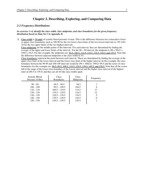
Chapter 2: Describing, Exploring, and Comparing Data 7Chapter 2. Describing, Exploring, and Comparing Data2-2 Frequency DistributionsIn exercises 1–4, identify the class width, class midpoints, and class boundaries for the given frequencydistribution based on Data Set 1 in Appendix B.1. Class width is 10 units of systolic blood pressure of men. This is the difference between two consecutive loweror upper class boundaries such as 100-90 for the two lower class limits of the two lowest intervals or 159-149=10 for the two upper limits of the two highest intervals.Class midpoints are the middle points of the intervals. For each interval, they are determined by finding theaverage of the upper and lower limits of the interval. For the 90 – 99 interval, the midpoint is (90 + 99)/2 =189/2 = 94.5. For this example, the midpoints are: 94.5, 104.5, 114.5, 124.5, 134.5, 144.5, and 155.5. Note thatthe difference between adjacent midpoints is the class width of 10.Class boundaries represent the point between each interval. These are determined by finding the average of theupper class limit of the lower interval and the lower class limit of the higher interval. In this example, the classboundary between the 90-99 and 100-109 intervals would be (99 + 100)/2= 199/2= 99.5 and the series of classboundaries for this example are: 89.5, 99.5, 109.5, 119.5, 129.5, 139.5, 149.5, and 159.5. Note that all the scoresfall in the range of the lower class boundary of the lowest interval and the higher class interval of the highestinterval (89.5 to 159.5) and they are all 10 (the class width) apart.Systolic BloodPressure of MenClassBoundariesClassMidpointsFrequency90 – 99100 – 109110 – 119120 – 129130 – 139140 – 149150 – 15989.5 – 99.599.5 – 109.5109.5 – 119.5119.5 – 129.5129.5 – 139.5139.5 – 149.5149.5 – 159.594.5104.5114.5124.5134.5144.5155.5141712501

8 Chapter 2: Describing, Exploring, and Comparing Data2. Class width is 20 units of systolic blood pressure of women. This is the difference between two consecutivelower or upper class boundaries such as 100-80 for the two lower class limits of the two lowest intervals or 199-179= 20 for the two upper limits of the two highest intervals.Class midpoints are the middle points of the intervals. For each interval, they are determined by finding theaverage of the upper and lower limits of the interval. For the 80 – 99 interval, the midpoint is (80 + 99)/2 =179/2 = 89.5. For this example, the midpoints are: 89.5, 109.5, 129.5, 149.5, 169.5, and 189.5. Note that thedifference between adjacent midpoints is the class width of 20.Class boundaries represent the point between each interval. These are determined by finding the average of theupper class limit of the lower interval and the lower class limit of the higher interval. In this example, the classboundary between the 80-99 and 100-119 intervals would be (99 + 100)/2= 199/2= 99.5 and the series of classboundaries for this example are: 79.5, 99.5, 119.5, 139.5, 159.5, 179.5, and 199.5. Note that all the scores fall inthe range of the lower class boundary of the lowest interval and the higher class interval of the highest interval(79.5 to 199.5) and they are all 20 units of systolic blood pressure (the class width) apart.Systolic Blood Pressureof WomenClassBoundariesClassMidpointsFrequency80 – 99100 – 119120 – 139140 – 159160 – 179180 – 19979.5 – 99.599.5 – 119.5119.5 – 139.5139.5 – 159.5159.5 – 179.5179.5 – 199.589.5109.5129.5149.5169.5189.592451013. Class width is 200 units of cholesterol of men. This is the difference between two consecutive lower or upperclass boundaries such as 0-200 for the two lower class limits of the two lowest intervals or 1200-1000= 200 forthe two upper limits of the two highest intervals.Class midpoints are the middle points of the intervals. For each interval, they are determined by finding theaverage of the upper and lower limits of the interval. For the 0 – 199 interval, the midpoint is (0 + 199)/2 =199/2 = 99.5. For this example, the midpoints are: 99.5, 299.5, 499.5, 699.5, 899.5, 1099.5 and 1299.5. Notethat the difference between adjacent midpoints is the class width of 200.Class boundaries represent the point between each interval. These are determined by finding the average of theupper class limit of the lower interval and the lower class limit of the higher interval. In this example, the classboundary between the 0 – 199 and 200 – 399 intervals would be (199 + 200)/2= 399/2= 199.5 and the series ofclass boundaries for this example are: -0.5, 199.5, 399.5, 599.5, 799.5, 999.5, 1199.5, and 1399.5. Note that allthe scores fall in the range of the lower class boundary of the lowest interval and the higher class interval of thehighest interval (199.5 to 1399.5) and they are all 200 units of cholesterol (the class width) apart.Cholesterol of Men0 – 199200 – 399400 – 599600 – 799800 – 9991000 – 11991200 – 1399ClassBoundaries-0.5 – 199.5199.5 – 399.5399.5 – 599.5599.5 – 799.5799.5 – 999.5999.5 – 1199.51199.5 – 1399.5ClassMidpoints99.5299.5499.5699.5899.51099.51299.5Frequency131158201

Chapter 2: Describing, Exploring, and Comparing Data 94. In this case, the observations are not whole numbers, but are fractional ones, measured to the nearest tenth of ascore.Class width is 6 units of body mass units of women. This is the difference between two consecutive lower orupper class boundaries such as 15.0 – 21.0 for the two lower class limits of the two lowest intervals or 44.9 –38.9= 6 for the two upper limits of the two highest intervals.Class midpoints are the middle points of the intervals. For each interval, they are determined by finding theaverage of the upper and lower limits of the interval. For the 15.0 – 20.9 interval, the midpoint is (15.0 + 20.9)/2= 35.9/2 = 17.95. For this example, the midpoints are: 17.95, 23.95, 29.95, 35.95, and 41.95. Note that thedifference between adjacent midpoints is the class width of 6.Class boundaries represent the point between each interval. These are determined by finding the average of theupper class limit of the lower interval and the lower class limit of the higher interval. In this example, the classboundary between the 15.0-20.9 and 21.0-26.9 intervals would be (20.9 + 21.0)/2= 41.9/2= 20.95 and the seriesof class boundaries for this example are: 14.95, 20.95, 26.95, 32.95, 38.95, and 44.95. Note that all the scoresfall in the range of the lower class boundary of the lowest interval and the higher class interval of the highestinterval (14.95 to 44.95) and they are all 6 units of body mass index (the class width) apart.Body Mass Indexof WomenClassBoundariesClassMidpointsFrequency15.0 – 20.921.0 – 26.927.0 – 32.933.0 – 38.939.0 – 44.914.95 – 20.9520.95 – 26.9526.95 – 32.9532.95 – 38.9538.95 – 44.9517.9523.9529.9535.9541.9510151122In exercises 5–8, construct the relative frequency distributions that correspond to the frequency distribution inthe exercise indicated.The relative frequency is the proportion, usually converted to a percent, of scores in each interval, the equationto be used is:Class frequencyRelative frequency =Sum of all frequencies5. For Systolic Blood Pressure of Men (Exercise 1), the sum of frequencies (n) is 40For the 90 – 99 interval, relative frequency = 1/40 * 100% = 0.025 * 100%= 2.5%For the 120 – 129 interval, relative frequency = 12/40 * 100% = 0.30 * 100%= 30.0%Systolic Blood Pressureof Men90 – 99100 – 109110 – 119120 – 129130 – 139140 – 149150 – 159Frequency141712501RelativeFrequency2.5%10.0%42.5%30.0%12.5%0.0%2.5%

10 Chapter 2: Describing, Exploring, and Comparing Data6. For Systolic Blood Pressure of Women (Exercise 2), the sum of frequencies (n) is 40For the 80 – 99 interval, relative frequency = 9/40 * 100% = 0.225 * 100%= 22.5%For the 100 – 119 interval, relative frequency = 24/40 * 100% = 0.60 * 100%= 60.0%Systolic Blood Pressureof Women80 – 99100 – 119120 – 139140 – 159160 – 179180 – 199Frequency9245101RelativeFrequency22.5%60.0%12.5%2.5%0.0%2.5%7. For Cholesterol of Men (Exercise 3), the sum of frequencies (n) is 40.For the 200 – 399 interval, relative frequency is 11/40 * 100% = 0.275 * 100%= 27.5%For the 1200 – 1399 interval, relative frequency is 1/40 * 100% = 0.025 * 100= 2.50%Cholesterol of Men0 – 199200 – 399400 – 599600 – 799800 – 9991000 – 11991200 – 1399Frequency131158201RelativeFrequency32.5%27.5%12.5%20.0%5.0%0.0%2.5%8. For Body Mass Index of Women (Exercise 4), the sum of frequencies (n) is 40For the 15.0 – 20.9 interval, relative frequency is 10/40 * 100% = 0.25 * 100%= 25.0%For the 33.0 – 38.9 interval, relative frequency is 2/40 * 100% = 0.05 * 100%= 5.0%Body Mass Indexof Women15.0 – 20.921.0 – 26.927.0 – 32.933.0 – 38.939.0 – 44.9Frequency10151122RelativeFrequency25.0%37.5%27.5%5.0%5.0%In exercises 9-12, construct the cumulative frequency distribution that corresponds to the frequency distributionin the exercise indicated.The cumulative frequency in each interval is the sum of the frequencies in the interval and all of the frequenciesin the intervals below (in score terms) that interval. Cumulative frequency in the highest score interval mustequal the sum of all frequencies (n).

Chapter 2: Describing, Exploring, and Comparing Data 119. For Systolic Blood Pressure of Men (Exercise 5)Systolic Blood Pressureof Men90 – 99100 – 109110 – 119120 – 129130 – 139140 – 149150 – 159Frequency141712501Workingcolumn (not infinal table)f in interval +cumulative f upto interval1 + 0 = 14 + 1 = 517 + 5 = 2212 + 22 = 345 + 34 = 390 + 39 =3939 + 1 = 40CumulativeFrequency15223439394010. For Systolic Blood Pressure of Women (Exercise 6)Systolic Blood Pressureof Women80 – 99100 – 119120 – 139140 – 159160 – 179180 – 199Frequency9245101Workingcolumn (not infinal table)f in interval +cumulative f upto interval9 + 0 = 924 + 9= 335 + 33 = 381 + 38= 390 + 39= 391 + 39 = 40CumulativeFrequency9333839394011. For Cholesterol of Men (Exercise 7)Cholesterol of Men0 – 199200 – 399400 – 599600 – 799800 – 9991000 – 11991200 – 1399Frequency131158201Workingcolumn (not infinal table)f in interval +cumulative f upto interval0 + 13 = 1311 + 13 = 245 + 24= 298 + 29 = 372 + 37 = 390 + 39 = 391 + 39 = 40CumulativeFrequency13242937393940

12 Chapter 2: Describing, Exploring, and Comparing Data12. For Body Mass Index of Women (Exercise 8)Body Mass Indexof WomenFrequencyWorkingcolumn (not infinal table)f in interval +cumulative f upto intervalCumulativeFrequency15.0 – 20.921.0 – 26.927.0 – 32.933.0 – 38.939.0 – 44.91015112210 + 0 = 1015 + 10 = 2511 + 25= 362 + 36 = 382 + 38 = 40102536384013. Bears Frequency Distribution of Weight of Bears in Pounds (From Data Set 6)Weight ofBears in FrequencyPounds0 – 49 650 – 99 10100 –149 10150 –199 7200 – 249 8250 – 299 2301 – 349 4350 – 399 3400 – 449 3450 – 499 0500 – 549 114. Body Temperatures (From Data Set 2)Body Temperatureat Midnight of Second FrequencyDay96.5 – 96.8 196.9 – 97.2 897.3 – 97.6 1497.7 – 98.0 2298.1 – 98.4 1998.5 – 98.8 3298.9 − 99.2 699.3 – 99.6 4Two notable things about this frequency distribution are: 1. that the scale of the classes does not include all ofthe scores since there are four scores that are not included in the range of classes selected and 2. The intervalscould have been made shorter (say 3 o F) so the distribution could have been spread out more. With this manyscores (n= 106), more intervals might have given a better detail of the nature of the distribution.

Chapter 2: Describing, Exploring, and Comparing Data 1315. Head Circumferences in cm. of Two-Month-Old Babies (From Data Set 4)HeadCircumference incm.Frequency ofMalesFrequencyof Females34.0 – 35.9 2 136.0 – 37.9 0 338.0 – 39.9 5 1440.0 – 41.9 29 2742.0 – 43.9 14 5From the comparison of the two frequency distributions, it seems that the head circumference for the malebabies is higher than for the female babies. However, we cannot conclude that the difference is statisticallysignificant until we conduct specific tests to test these differences.16. Very Poplar Trees Weights in kg. (From Data Set 9)Poplar Weights inkg.Frequencyfor Year 20.00 - 0.49 70.50 - 0.99 151.00 - 1.49 101.50 - 1.99 72.00 - 2.49 117. Yeast Cell Counts (From Data Set 11)YeastCell FrequencyCounts1 202 433 534 865 706 547 378 189 1010 511 212 2The most common cell count is 4 with a frequency of 86.18. Number of Classes Using Sturges’ guideline, n represents the number of data values and x represents thenumber of classesx = 1+(log n) /(log 2)n = 2 x−1We will need to find values where there are lower and upper limits associated with determined numbers of datavalues. If we are looking for values related to having 5 to 12 classes, we need an upper and lower limit for each

14 Chapter 2: Describing, Exploring, and Comparing Dataof these. For 5 this will be 4.5 to 5.5, for 6 this will be 5.5 to 6.5, and so on until the last category would have 12classes and 11.5 to 12.5 will be used for the limits. The number of values at each limit is determined by:n = 2 x−1where x are the limits.We can display this in the following table:Number of classes(x)Lower and Upper xLimitsNumber of Values at Lowerand Upper Limitsn = 2 x-1Number ofValues(Rounded)567891011124.5 – 5.55.5 – 6.56.5 – 7.57.5 – 8.58.5 – 9.59.5 – 10.510.5 – 11.511.5 – 12.511.31 – 22.6322.63 – 45.2545.25 – 90.5190.51 – 181.02181.02 – 362.04362.04 – 724.08724.08 – 1448.151448.15 – 2896.3111 – 2223 – 4546 – 9091 – 181182 – 362363 – 724725 – 14481449 - 28962-3 Visualizing DataIn Exercises 1-4, answer the questions by referring to the SPSS-generated histogram given below. The histogramrepresents the lengths (mm) of cuckoo eggs found in the nests of other birds (based on data from O.M. Latter andData and Story Library).1. Center Center is a very general term, but basically it looks for a central value that could be used to represent theentire distribution. One value that could be used is the center of the scale which would be at the average of thelow (19.75) and high (24.76) points, which would be (19.75 + 24.76)/2= 22.25 mm of egg length. Anotherpossible value for center would be the value that occurs most often which would be taken as the midpoint of the22.0 interval. One statistic that is reported in the table is the mean of 22.46 mm. This is one of the descriptivestatistics that is often used to represent the center of a continuous distribution.2. Variation For these data, the lowest possible egg length would be the lowest score limit in the lowest interval.That interval is the 19.625 to 19.875 interval and the lowest possible score in that interval is 19.625 mm. Thehighest possible egg length would be the highest score limit in the highest interval. That interval is the 24.875to 25.125 interval and the highest possible score in that interval is 25.125 mm. Thus, the range of observed eggvalues is 19.625 to 25.125.3. Percentage Note the midpoints of the intervals are not all labeled. There are three intervals that have midpointsof 20.75, 21.00, and 21.25 (21.00 is not printed, but it is there). The lower and upper limits of these threeintervals are: 20.625 – 20.875, 20.875 – 21.125, and 21.125 – 21.375. 21.125 is the upper limit of the 20.875to 21.125 interval. Therefore, all of the eggs in that interval and below are less than 21.125 mm. Counting themfrom the start up though that interval, we have 2 + 2 + 1 + 0 + 6 + 6 = 17 and that equates to a percentage of17/120 (100%) = 14.2%.4. Class width The easiest way to find this is to find the difference between midpoints of two adjacent intervals.As we saw in exercise three, there were three adjacent intervals with midpoints of 20.75, 21.00, and 21.25. Eachof these midpoints is 0.25 mm different from adjacent intervals, the class width is 0.25 mm.In Exercises 5 and 6, refer to the accompanying pie chart of blood groups for a large sample of people (based ondata from the Greater New York Blood Program).5. Interpreting Pie Chart It would appear that about 40% of the observed group has Group A blood and out of500 in the sample, this would be about 200 people.

Chapter 2: Describing, Exploring, and Comparing Data 156. Interpreting Pie Chart It appears that about 10% of the observed group has Group B blood and out of 500 inthe sample, this would be about 50 people.7. Bears Histogram of Weights in PoundsWeight of Bears in Pounds12108Frequency642024.5 74.5 124.5 174.5 224.5 274.5 324.5 374.5 424.5 474.5 524.5Weight in PoundsThe approximate weight at the center seems to be between 174.5 and 224.5 or about 200 pounds. We couldcompute the mean and find it is 183 pounds, which would be a useful measure of centrality of the distribution.8. Body Temperatures in Degrees Fahrenheit Histogram (Data Set 2)Body Temperatures at Midnight of Second Day353025Frequency2015105096.5 96.9 97.3 97.7 98.1 98.5 98.9 99.3Temperature in Degrees F98.6 o F seems close to where we would expect the mean of this distribution to be. However, there is somevariation around that value. This does not appear to be a bell-shaped distribution. It is skewed toward the lowerend of the scale, which we would describe as being negatively skewed.

16 Chapter 2: Describing, Exploring, and Comparing Data9. Yeast Cell Counts Histogram (Data Set 11)Yeast Cell Counts10090807060Frequency504030201001 2 3 4 5 6 7 8 9 10 11 12Number of Yeast Cells over 1 mm2The distribution seems to depart somewhat from being bell-shaped. It seems to have a reasonable degree ofpositive skewness. Other specific measures can be used to assess the exact degree of skewness.In Exercises 10 and 11, use graphs to compare the two indicated data sets.10. Head Circumferences (Data Set 4), Frequency Polygons for Males and FemalesHead Circumferences of Two-Month-OldsComparison of Males and Females353025Frequency2015MalesFemales105034.9 36.9 38.9 40.9 42.9 44.9 46.9Head Circumference in cm.From the frequency polygon, it would appear that the head circumference for males is slightly higher than thatfor females. However, to determine statistical significance, we would need to conduct other tests designed to aidin making those decisions.

Chapter 2: Describing, Exploring, and Comparing Data 1711. Poplar Trees Histogram comparing Heights (in meters) of Control Group and Irrigation Only Trees (From DataSet 9)Comparison of Control and Irrigation Treatment Height of Poplar Trees543FrequencyControlTreatment2101.5 2 2.5 3 3.5 4 4.5 5 5.5 6 6.5 MoreHeight of Poplar Trees in MetersThe two distributions do not seem to have much departure from each other and this would not seem to beenough for us to conclude that the distributions are significantly different. There is no sound evidence toconclude that the irrigation treatment had any effect on poplar tree height.In Exercises 12 and 13, list the original data represented by the given stem-and-leaf plots.12. To find the original score, the leaf (in units of one) is added to the stem which is in units of tens. The originaldata displayed in stem-and-leaf plot would be:200 200 200 205 216 219 219 219 219 222 222 223 223 223 223 223241 241 247 24713. To find the original scores, the leaf in units of tens and ones is added to the stem which is in units of hundreds.5012 5012 5012 5055 5200 5200 5200 5200 5327 5327 5335 5472

18 Chapter 2: Describing, Exploring, and Comparing DataIn Exercises 14 and 15, construct the dotplot for the data represented by the stem-and-leaf plot in the givenexercise.14. Dotplot of Exercise 12 DataDotplot of Data in Exercise 2-3 12654Frequency32115. Dotplot of Exercise 13 Data0198 200 202 204 206 208 210 212 214 216 218 220 222 224 226 228 230 232 234 236 238 240 242 244 246 248Variable ValueDotplot of Data in Exercise 2-3 13543Frequency2105000 5025 5050 5075 5100 5125 5150 5175 5200 5225 5250 5275 5300 5325 5350 5375 5400 5425 5450 5475 5500Variable Value16. Construct Stem-and-Leaf Plot for Exercise 11.Data points are:4.1 2.5 4.5 3.6 2.8 5.1 2.9 5.1 1.2 1.6 6.4 6.8 6.5 6.8 5.8 2.9 5.5 3.3 6.1 6.1

Chapter 2: Describing, Exploring, and Comparing Data 19First, put them in order:1.2 1.6 2.5 2.8 2.9 2.9 3.3 3.6 4.1 4.5 5.1 5.1 5.5 5.8 6.1 6.1 6.4 6.5 6.8 6.8Stem will be in units of ones and leaf will be in units of tenths, need stems that range from 1 to 6Stem(units)1.2.3.4.5.6.Leaves(tenths)26589936151158114588In Exercises 17-20, use the given paired data from Appendix B to construct a scatter diagram.17. Parent/Child Height (Data Set 3)To determine a relationship graphically, we will use a scatter diagram with mother’s height on the horizontal (xaxis)scale and the child’s height on the vertical (y-axis) scale.Scatter Diagram of Child and Mother Heights, in Inches7570Child's Height65605555 60 65 70 75Mother's HeightThere appears to be a relationship and the nature of the relationship is that low heights on both cluster togetherand high heights on both cluster together or another way of saying this is that as height on one increases weobserve height on the other increasing, also called a direct or positive relationship.

20 Chapter 2: Describing, Exploring, and Comparing Data18. Bear Neck/Weight (Data Set 6)Scatter Diagram of Bear Neck Size and Weight600500400Weight in lb.30020010000 5 10 15 20 25 30 35Neck Size in InchesThere is a general positive relationship. As neck size increases, we observe an increase in weight.19. Sepal/Petal Length (Data Set 7)Scatter Diagram of Setosa Class Sepal and Petal Lengths21.91.81.71.6Petal Length in mm.1.51.41.31.21.110.90.84 4.5 5 5.5 6Sepal Length in mm.There does not appear to be a relationship between sepal length and petal length for the Setosa Class. As one ofthe variables changes in a given direction, there seems to be no corresponding change in the other variable ineither direction.

Chapter 2: Describing, Exploring, and Comparing Data 2120. Red and White Blood Counts (Data Set 10)Scatter Diagram of Red and White Blood Counts6.56Red Blood Count in Cells/Microliter5.554.543.530 2 4 6 8 10 12 14 16 18White Blood Count in Cells/MicroliterThere does not appear to be a relationship between red and white blood count. As one of the variables changesin a given direction, there seems to be no corresponding change in the other variable in either direction.2-4 Measures of CenterIn Exercises 1-8, find the (a) mean, (b) median, (c) mode, and (d) midrange for the given sample data.The four measures of center used below are:a. the mean ( x ) which we find using the following equation:Mean: x ∑xn where∑= / x represents the sum of scoresb. the median ( x ~ ) which is determined with the following rules:If there are an odd number of scores, the median is the score that is exactly in themiddle of the ordered set of scores.If there are an even number of scores, the median is the point exactly between or theaverage of the two middle scores.c. the mode, which is the score that occurs most often; if there are two that occur most often thatare tied, the distribution is bimodal and two modes are reported; if there are three that occur most often thatare tied, the distribution is trimodal and three modes are reported; if no score occurs more often than anyothers or if there are more than three that occur most often and they are tied, no mode is reported.d. the midrange is the point exactly between or the average of the lowest and highest scores1. Tobacco Use in Children’s Movies Arranged in order, the scores are:# 1 2 3 4 5 6Score 0 0 0 176 223 548a. Mean: x = ∑ x / n = 947 / 6 = 157. 8b. Median: x ~ is the midpoint between the two middle scores (3 rd and 4 th scores) if an even number of scores.This would be (0 + 176)/2= 176/2= 88.0

22 Chapter 2: Describing, Exploring, and Comparing Datac. Mode: Mode is score that occurs most often, this is 0 for these datad. Midrange: Midpoint (or average) between lowest and highest scores, (548 + 0)/2 = 548/2=274.02. Cereal Arranged in order, the scores are# 1 2 3 4 5 6 7 8 9 10 11 12 13 14 15 16Score .03 .07 .09 .13 .13 .17 .24 .30 .39 .43 .43 .44 .45 .47 .47 .48a. Mean: x = ∑ x / n = 4.72 /16 = 0. 295b. Median: ~ x is the midpoint between the two middle scores (8 th and 9 th scores) if an even number of scores.This would be (0.30 + 0.39)/2= 0.69/2= 0.345c. Mode: Mode is score that occurs most often, there are three scores that occur most often so the distributionis tri-modal at 0.13, 0.43, and 0.47d. Midrange: Midpoint (or average) between lowest and highest scores, (0.48 + 0.03)/2 = 0.51/2= 0.255. Is themean likely to be a good estimate of the mean amount of sugar in each gram of cereal consumed by thepopulation of all Americans who eat cereal? The sample mean is always the best estimate of the populationmean. However, since the distribution is skewed (negatively), the median might be a better center estimateof the amount of sugar in each gram of cereal consumed by the population of all Americans who eat cereal.3. Body Mass Index Arranged in order, the scores are:# 1 2 3 4 5 6 7 8 9 10 11 12Score 17.7 19.6 19.6 20.6 21.4 22.0 23.8 24.0 25.2 27.5 28.9 29.1# 13 14 15Score 29.9 33.5 37.7a. Mean: x = ∑ x / n = 380.5/15 = 25. 37b. Median: ~ x is the middle score (8 th score) if an odd number of scores. This would be 24.0c. Mode: Mode is score that occurs most often, the only score that occurs more than once is 19.6 so that is themoded. Midrange: Midpoint (or average) between lowest and highest scores, (37.7 + 17.7)/2 = 20.0/2= 27.7Is the mean of this sample reasonably close to the mean of 25.74, which is the mean for all 40 women includedin Data Set 1? Yes, they are very close, especially when on considers the range of values to be from about 17 to38.4. Drunk Driving Arranged in order, the scores are:# 1 2 3 4 5 6 7 8 9 10 11 12 13 14 15Score .12 .13 .14 .16 .16 .16 .17 .17 .17 .18 .21 .24 .24 .27 .29a. Mean: x = ∑ x / n = 2.81/15 = 0. 187b. Median: ~ x is the middle score (8 th score) if an odd number of scores. This would be 0.17

Chapter 2: Describing, Exploring, and Comparing Data 23c. Mode: Mode is score that occurs most often. In this case two scores occur three times (0.16 and 0.17) andsince these are adjacent to each other in the order, the mode is taken as the midpoint between them, so themode in this case would be 0.165)d. Midrange: Midpoint (or average) between lowest and highest scores, (0.29 + 0.12)/2 = 0.41/2= 0.2055. Motorcycle Fatalities Arranged in order, the scores are:# 1 2 3 4 5 6 7 8 9 10 11 12 13 14 15Score 14 16 17 18 20 21 23 24 25 27 28 30 31 34 37# 16 17 18Score 38 40 42a. Mean: x = ∑ x / n = 485/18 = 26. 9b. Median: ~ x is the average of the middle scores (9 th and 10 th scores) if an even number of scores. This wouldbe (25 + 27)/2= 52/2= 26.0c. Mode: Mode is score that occurs most often. In this case no score occurs more than once so there is no moded. Midrange: Midpoint (or average) between lowest and highest scores, (14 + 42)/2 = 56/2= 28.0Do the results support the common belief that such fatalities are incurred by a greater proportion of youngerdrivers? Following is a histogram of the frequencies:Age of Motorcycle Fatalities from US Dept. of Transportation543Frequency21015 20 25 30 35 40 45AgeIn the range of ages of fatalities for these data, the distribution is fairly even from ages 14 to 42, with a slightlyhigher distribution toward the lower range, but not such a distinct difference that would warrant concluding thatsuch fatalities are incurred by a greater proportion of younger drivers. It is difficult to answer this question sincewe don’t know and might reasonable question whether there would be an equal proportion of motorcycle ridersacross all the age groups. Also, this data set is relatively small to permit making such a conclusion.

24 Chapter 2: Describing, Exploring, and Comparing Data6. Fruit Flies Arranged in order, the scores are:# 1 2 3 4 5 6 7 8 9 10 11Score 0.64 0.68 0.72 0.76 0.84 0.84 0.84 0.84 0.90 0.90 0.92a. Mean: x = ∑ x / n = 8.88 /11 = 0. 807b. Median: ~ x is the middle score (6 th ) if an odd number of scores. This would be 0.84c. Mode: Mode is score that occurs most often. In this case the mode is 0.84 since that occurs most oftend. Midrange: Midpoint (or average) between lowest and highest scores, (0.64 + 0.92)/2 = 1.56/2= 0.787. Blood Pressure Measurements Arranged in order, the scores are:# 1 2 3 4 5 6 7 8 9 10 11 12 13 14Score 120 120 125 130 130 130 130 135 138 140 140 143 144 150a. Mean: x = ∑ x / n = 1875 /14 = 133. 9b. Median: ~ x is the midpoint between the two middle scores (7 th and 8 th scores) if an even number of scores.This would be (130 + 135)/2= 265/2= 132.5c. Mode: Mode is score that occurs most often. In this case the mode is 130 since that occurs most often (4times)d. Midrange: Midpoint (or average) between lowest and highest scores, (120 + 150)/2 = 270/2= 135What is notable about this data set? The measures of centrality are relatively close, which would indicate thedistribution seems relatively symmetrical.8. Phenotypes of Peas Arranged in order, the scores are:# 1 2 3 4 5 6 7 8 9 10 11 12 13 14 15Score 1 1 1 1 1 1 1 1 1 1 1 2 2 2 2# 16 17 18 19 20 21 22 23 24 25Score 2 2 2 3 3 3 3 3 3 4a. Mean: x = ∑ x / n = 47 / 25 = 1. 88b. Median: ~ x is the middle score (13 th ) if an odd number of scores. This would be 2.0c. Mode: Mode is score that occurs most often. In this case, 1 occurs more than any other score (11 times) sothe mode is 1.0d. Midrange: Midpoint (or average) between lowest and highest scores, (1 + 4)/2 = 5/2= 2.5The level of measurement is ordinal since the categories can be ranked or ordered. Measure of center can beobtained for these values. Do the results make sense? While central measures are often used with ordinal data,the fact that they do not have equal intervals would make the mean of questionable use, but the median andmode might be useful.

Chapter 2: Describing, Exploring, and Comparing Data 25In Exercises 9-12, find the mean, median, mode, and midrange for each of the samples then compare the two setsof results.9. Patient Waiting TimesSingle Line Central Statistics: Arranged in order, the scores are:# 1 2 3 4 5 6 7 8 9 10Score 65 66 67 68 71 73 74 77 77 77a. Mean: x = ∑ x / n = 715 /10 = 71. 5b. Median: ~ x is the midpoint between the two middle scores (5 th and 6 th scores) if an even number of scores.This would be (71 + 73)/2= 144/2= 72.0c. Mode: Mode is score that occurs most often. In this case the mode is 77 since that occurs most oftend. Midrange: Midpoint (or average) between lowest and highest scores, (65 + 77)/2 = 142/2= 71.0Multiple Line Central Statistics: Arranged in order, the scores are:# 1 2 3 4 5 6 7 8 9 10Score 42 54 58 62 67 77 77 85 93 100a. Mean: x = ∑ x / n = 715 /10 = 71. 5b. Median: ~ x is the midpoint between the two middle scores (5 th and 6 th scores) if an even number ofscores. This would be (67 + 77)/2= 144/2= 72.0c. Mode: Mode is score that occurs most often. In this case the mode is 77 since that occurs most oftend. Midrange: Midpoint (or average) between lowest and highest scores, (42 + 100)/2 = 142/2= 71Comparison of the two distributions relative to central measures: The central measures are exactly the same forboth groups. However, there is more spread of the scores from each other for the multiple line group (42 to 100)compared with the single line group (65 to 77).10. Skull Breadths4000 B. C. Central Statistics: Arranged in order, the scores are:# 1 2 3 4 5 6 7 8 9 10 11 12Score 119 125 126 126 128 128 129 131 131 131 132 138a. Mean: x = ∑ x / n = 1544 /12 = 128. 7b. Median: ~ x is the midpoint between the two middle scores (6 th and 7 th scores) if an even number of scores.This would be (128 + 129)/2= 257/2= 128.5c. Mode: Mode is score that occurs most often. In this case the mode is 131 since that occurs most often (3times)d. Midrange: Midpoint (or average) between lowest and highest scores, (119 + 138)/2 = 257/2= 128.5

26 Chapter 2: Describing, Exploring, and Comparing Data150 A. D. Central Statistics: Arranged in order, the scores are:# 1 2 3 4 5 6 7 8 9 10 11 12Score 126 126 129 130 131 133 134 136 137 138 139 141a. Mean: x = ∑ x / n = 1600 /12 = 133. 3b. Median: ~ x is the midpoint between the two middle scores (6 th and 7 th scores) if an even number of scores.This would be (133 + 134)/2= 267/2= 133.5c. Mode: Mode is score that occurs most often. In this case the mode is 126 since that occurs most often (2times)d. Midrange: Midpoint (or average) between lowest and highest scores, (126 + 141)/2 = 267/2= 133.5Comparison of the two distributions relative to central measures: The central measures are slightly higher on allcentral measures except the mode (which tends to be less stable as a measure compared with the others) for the150 A. D. sample than for the 4000 B.C. group. Head sizes appear to have gotten larger between 4000 B C. and150 A. D. However, it is not valid to attribute such change to interbreeding with people from other regions.These data provide no basis for making such a conclusion as to any cause for this change.11. Poplar TreesControl Group Central Statistics: Arranged in order, the scores are:# 1 2 3 4 5 6 7 8 9 10 11 12 13 14 15Score 1.9 2.9 3.2 3.6 3.9 4.1 4.1 4.6 4.8 4.9 5.1 5.5 5.5 5.5 6.0# 16 17 18 19 20Score 6.3 6.5 6.8 6.9 6.9a. Mean: x = ∑ x / n = 99.0 / 20 = 4. 95b. Median: ~ x is the midpoint between the two middle scores (10 th and 11 th scores) if an even number ofscores. This would be (4.9 + 5.1)/2= 10.0/2= 5.0c. Mode: Mode is score that occurs most often. In this case, 5.5 occurs more than any other score (3 times) sothe mode is 5.5d. Midrange: Midpoint (or average) between lowest and highest scores, (1.9 + 6.9)/2 = 8.8/2= 4.4Irrigation Treatment Group Central Statistics: Arranged in order, the scores are:# 1 2 3 4 5 6 7 8 9 10 11 12 13 14 15Score 1.2 1.6 2.5 2.8 2.9 2.9 3.3 3.6 4.1 4.5 5.1 5.1 5.5 5.8 6.1# 16 17 18 19 20Score 6.1 6.4 6.5 6.8 6.8a. Mean: x = ∑ x / n = 89.6 / 20 = 4. 48b. Median: ~ x is the midpoint between the two middle scores (10 th and 11 th scores) if an even number ofscores. This would be (4.5 + 5.1)/2= 9.6/2= 4.80c. Mode: Mode is score that occurs most often. In this case, 4 scores occur the same number of times (twice)so the distribution has four modes with modes at: 2.9, 5.1, 6.1 and 6.8 occurs more than any other score (3times) so there is no distinct mode

Chapter 2: Describing, Exploring, and Comparing Data 27d. Midrange: Midpoint (or average) between lowest and highest scores, (1.2 + 6.8)/2 = 8.0/2= 4.0Comparison of the two distributions relative to central measures: The central measures are slightly higher on themean and the median for the control group on the heights (in meters) of the trees.12. Poplar TreesThe breakout of the stem and leaf plot provides the score data which are arranged in order below:# 1 2 3 4 5 6 7 8 9 10 11 12 13 14 15Score 3.2 3.9 4.4 5.4 6.3 6.3 6.4 6.7 6.8 6.8 6.9 6.9 6.9 7.1 7.3# 16 17 18 19 20Score 7.3 7.3 7.6 7.7 8.0a. Mean: x = ∑ x / n = 129.2 / 20 = 6. 46 (Control Group Mean= 4.95)b. Median: ~ x is the midpoint between the two middle scores (10 th and 11 th scores) if an even number ofscores. This would be (6.8 + 6.9)/2= 13.7/2= 6.85 (Control Group Median= 5.0)c. Mode: Mode is score that occurs most often (4 times). In this case, 2 scores occur more than any others sothere are two modes: 6.9 and 7.3 (Control Group Mode= 5.5)d. Midrange: Midpoint (or average) between lowest and highest scores, (3.2 + 8.0)/2 = 11.2/2= 5.6 (ControlGroup Midrange= 4.4)Comparison with Control Group. All central measures of tree height are higher for the trees that receivedfertilizer and irrigation when compared with the control group. Without more sophisticated tests we cannot tellwhether the difference is statistically significant, that is not likely to be attributable to chance.In Exercises 13-16, refer to the data set in Appendix B. Use computer software or a calculator to find the meansand medians, then compare the results as indicated.13. Head Circumference Comparison head circumference in cm. of males and females on central measures (DataSet 4)Statistic Males FemalesMean 41.10 40.05Median 41.10 40.20There does appear to be a slight difference since both central measures are higher for the males than for thefemales with males having a 1.05 cm. higher mean circumference.14. Body Mass Index Comparison of BMI of men and women (Data Set 1)Statistic Men WomenMean 26.00 25.74Median 26.20 23.90Yes, there does appear to be a slight difference since both central measures are higher for the men than for thewomen with men having a 0.26 BMI higher mean difference compared with the women. This may not be asignificant difference. We would need to determine this with other methods.

28 Chapter 2: Describing, Exploring, and Comparing Data15. Petal Lengths of Irises Comparison of petal lengths of the three classes (Data Set 7)Statistic Setosa Versicolor VirginicaMean 1.46 4.26 5.55Median 1.50 4.35 5.55No, they do not appear to have the same petal lengths. It is very clear that there are differences in centralmeasures among these three classes of Iris petal lengths. Petal length is much higher for the Versicolor andVirginica classes compared with the Setosa class while the length of the Virginica class seems to be higher thanthe length of petals for the Versicolor class. They may all be different from each other, but this would need tobe tested with more precise methods to decide.16. Sepal Widths of IrisesStatistic Setosa Versicolor VirginicaMean 3.42 2.77 2.97Median 3.40 2.80 3.00No, they do not appear to have the same sepal widths. There seems to be a difference between the Setosacompared with both the Versicolor and Virginica classes. There may be differences between the widths of theVersicolor and the Virginica classes as well. They may all be different from each other, but this would need tobe tested with more precise methods to decide.In Exercises 17 and 18, find the mean of the data summarized in the given frequency distribution.17. Mean from a Frequency Distribution The following frequency distribution will be used to find the goupedmean:Frequency Distribution of Cotinine Levels of SmokersSerumCotinine Level(mg/ml)Frequency(f)IntervalMidpoint(x)f ∗ x0 – 99100 – 199200 – 299300 – 399400 - 4991112141249.5149.5249.5349.5449.5544.51794.03493.0349.5899.0Sum Σf= 40 Σ(f ∗ x)= 7080.0∑(f∑∗ x)7080.0= =f 40Grouped Mean= 177. 0The mean computed using the actual raw values was 172.5.The Grouped Mean is close to the actual mean. The grouped mean is an estimate of the actual mean. With theavailability of computing equipment, the actual mean would be easy to compute and would always be preferred.However, if the raw scores were not available, this procedure could provide a reasonable estimate.

Chapter 2: Describing, Exploring, and Comparing Data 2918. Body Temperatures The following frequency distribution will be used to find the grouped mean:Frequency Distribution of Body TemperatureTemperature96.5 – 96.896.9 – 97.297.3 – 97.697.7 – 98.098.1 – 98.498.5 – 98.898.9 – 99.299.3 – 99.6Frequency(f)181422193264IntervalMidpoint(x)96.6597.0597.4597.8598.2598.6599.0599.45f ∗ x96.65776.401364.302152.701866.753156.80594.30397.80Sum Σf= 106 Σ(f ∗ x)= 10405.70∑(f∑∗ x)10405.70= =f 106Grouped Mean= 98. 17The mean computed using the actual raw values was 98.6 o F.The Grouped Mean is close to the actual mean, but underestimates it to some extent. The grouped mean is anestimate of the actual mean. With the availability of computing equipment, the actual mean would be easy tocompute and would always be preferred. However, if the raw scores were not available this procedure couldprovide a reasonable estimate.19. Mean of Means No, this process would not result in an accurate computation of the mean salary of physiciansfor the country. This process would provide a single mean entry per state in such a way that it would assumethe same number of physicians were in each state. Of course this is not true. There would be many morephysicians in states like New York and California compared with states like New Hampshire and Wyoming.The actual number of physicians within each state would need to be accounted for in this computation.20. Trimmed Meansa. The mean is 182.89 based on 54 scoresb. 10% trimmed mean (drop lowest 5 and highest 5 scores, based on 44 scores)= 171.00c. 20% trimmed mean (drop lowest 11 and highest 11 scores, based on 32 scores)= 159.16There are large differences among these three means when extreme score are removed. The mean decreaseswhen high extreme scores are removed (as in this example) and it increases when low extreme scores areremoved and if these are not distributed approximately equally below and above the mean, bias can occur.21. Censored Data The mean of the five values, including the one that is censored, would be 3.42. Since the twovalues of 5 are minimal values and their actual values would be higher than 5, we would conclude that the meanwould be 3.42 or higher.2-5 Measures of VariationIn Exercises 1-8, find the range, variance, and standard deviation for the given sample data (The same data wereused in Section 2 – 4 where we found measures of center. Here we find measures of variation).In the following computations of variance and standard deviation, the equation used to compute the varianceincludes the following terms:n represents the sample size

30 Chapter 2: Describing, Exploring, and Comparing Data∑ x represents the sum of the scores (the scores are added together)2)(∑ x represents the squared value for the sum of scores (the scores are added together and∑ 2then that value is squared)x represents the sum of the squared scores (each score is squared and then these are all added together)1. Tobacco Use in Children’s Movies. a. Range = highest score – lowest score = 548.0 – 0 = 548.0s222n( x ) − ( x)6(381009) − (947)=n(n −1)6(6 −1)1389245302b. Variance = = 46308. 2=∑ ∑2c. Standard Deviation s = s = 46308.2 = 215. 22. Cereala. Range = highest score – lowest score = 0.48 – 0.03 = 0.45s222n( x ) − ( x)16(1.8144) − (4.72)=n(n −1)16(16 −1)6.7522402b. Variance = = 0. 0281=∑ ∑2c. Standard Deviation s = s = 0.0281 = 0. 168Would an amount of sugar of 0.95 be considered “unusual”?Need to use the mean. From before it is 0.295 (Exercise 4.2)A sugar amount of 0.95 is not lower than the minimum usual value of mean – 2 s or0.295 – 2 (0.168)= 0.295 – 0.336 = – 0.041. But, a sugar amount of 0.95 is higher than the maximum usualvalue of mean + 2 s or 0.295 + 2 (0.168)= 0.295 + 0.336 = 0.631A sugar amount of 0.95 is NOT between the usual minimum and usual maximum values of– 0.041 and 0.631. Thus, a sugar amount of 0.95 would be considered unusual.3. Body Mass Indexa. Range = highest score – lowest score = 37.7 – 17.7 = 20.0s222n( x ) − ( x)15(10101.23) − (380.5)=n(n −1)15(15 −1)6738.202102b. Variance = = 32. 09=∑ ∑2c. Standard Deviation s = s = 32.0867 = 5. 66Would a body mass index of 34.0 be considered “unusual”?Need to use the mean. From before it is 25.37 (Exercise 4.3)A body mass index of 34 is not lower than the minimum usual value of mean – 2 s or25.37 – 2 (5.66) = 25.37 – 11.32 = 14.04 AND a body max index of 34 is not higher than the maximum usualvalue of mean + 2 s or 25.37 + 2 (5.66) = 25.37 + 11.32 = 36.69A body mass index of 34 is between the usual minimum and usual maximum values of 20.68 and 36.69. Thus,a body mass of 34 would not be considered unusual.4. Drunk Drivinga. Range = highest score – lowest score = 0.29 – 0.12 = 0.17

Chapter 2: Describing, Exploring, and Comparing Data 31s222n( x ) − ( x)15(0.5631) − (2.81)=n(n −1)15(15 −1)0.55042102b. Variance = = 0. 002621=∑ ∑2c. Standard Deviation s = s = 0.002621 = 0. 051When a state wages a campaign to reduce drunk driving, is the campaign intended to lower the standarddeviation? Such a campaign would be intended to reduce the variables such as number of crashes related todriving under the influence or the mean blood alcohol concentrations of drivers, not the standard deviation.5. Motorcycle Fatalitiesa. Range = highest score – lowest score = 42 – 14 = 28.0s222n( x ) − ( x)18(14343) − (485)=n(n −1)18(18 −1)229493062b. Variance = = 75. 00=∑ ∑2c. Standard Deviation s = s = 75.00 = 8. 66How does the variation of these ages compare to the variation of ages of all licensed drivers in the generalpopulation? The variation of this group will be lower since the range of 14 – 42 is lower than the typical rangeof the age of licensed drivers which would probably be from 15 to over 80. One would expect the variance andstandard deviation of this group to be lower as well.6. Fruit Fliesa. Range = highest score – lowest score = 0.92 – 0.64 = 0.28s222n( x ) − ( x)11(7.2568) − (8.88)=n(n −1)11(11−1)0.97041102b. Variance = = 0. 008822=∑ ∑2c. Standard Deviation s = s = 0.008822 = 0. 094Would a thorax length of 0.63 mm. be considered “unusual”?Need to use the mean. From before it is 0.807 (Exercise 2 – 4 .6)A thorax length of 0.63 mm. is not lower than the minimum usual value of mean – 2 s or0.807 – 2 (0.094) = 0.807 – 0.188 = 0.619 and a thorax length of 0.63 mm. is not higher than the maximumusual value of mean + 2 s or 0.807 + 2 (0.0.94) = 0.807 + 0.188 = 0.995A thorax length of 0.63 is between the usual minimum and usual maximum values of0.619 and 0.995. Thus, a thorax length of 0.63 would not be considered unusual.7. Blood Pressure Measurementsa. Range = highest score – lowest score = 150 – 120 = 30.0s222n( x ) − ( x)14(252179) − (1875)=n(n −1)14(14 −1)148811822b. Variance = = 81. 76=∑ ∑2c. Standard Deviation s = s = 81.76 = 9. 04

32 Chapter 2: Describing, Exploring, and Comparing DataWhat does this suggest about the accuracy of the readings? They do not appear to be very accurate when oneconsiders that all of these measures were taken on the same patient.8. Phenotypes of Peasa. Range = highest score – lowest score = 4 – 1 = 3.0s222n( x ) − ( x)25(109) − (47)=n(n −1)25(25 −1)5166002b. Variance = = 0. 860=∑ ∑2c. Standard Deviation s = s = 0.860 = 0. 927These are nominal data. Central and variation statistics can be computed on any set of numbers. However,since these data are nominal the statistics have no meaning. They are not legitimate since there is a lack ofequal intervals and no order to the categories.In Exercises 9-12, find the range, variance, and standard deviation for each of the two samples, then compare thetwo sets of results. (The same data were used in Section 2 – 4.)9. Patient Waiting TimesSingle line:a. Range = highest score – lowest score = 77 – 65 = 12.0s222n( x ) − ( x)10(51327) − (715)=n(n −1)10(10 −1)2045902b. Variance = = 22. 72=∑ ∑2c. Standard Deviation s = s = 22.72 = 4. 77Multiple line:a. Range = highest score – lowest score = 100 – 42 = 58.0s222n( x ) − ( x)10(54109) − (715)=n(n −1)10(10 −1)29865902b. Variance = = 331. 83=∑ ∑2c. Standard Deviation s = s = 331.83 = 18. 22Compare the results. There is clearly higher variation for the multiple line as compared with the single line.10. Skull Breadths4000 B.C.:a. Range = highest score – lowest score = 138 – 119 = 19s222n( x ) − ( x)12(198898) − (1544)=n(n −1)12(12 −1)28401322b. Variance = = 21. 515=∑ ∑2c. Standard Deviation s = s = 21.515 = 4. 64150 A.D.:a. Range = highest score – lowest score = 141 – 126 = 15

Chapter 2: Describing, Exploring, and Comparing Data 33s222n( x ) − ( x)12(213610) − (1600)=n(n −1)12(12 −1)33201322b. Variance = = 25. 152=∑ ∑2c. Standard Deviation s = s = 25.152 = 5. 02Compare the results. There is higher variation for the 150 A.D. group as compared with the 4000 B.C. group.Even though the range for the B.C. group is higher, the variance and standard deviations for the A.D. group ishigher and these are more accurate statistics since they use all of the scores rather than just two of them.11. Poplar TreesControl Group:a. Range = highest score – lowest score = 6.9 – 1.9 = 5.0s222n( x ) − ( x)20(528.42) − (99)=n(n −1)20(20 −1)767.403802b. Variance = = 2. 019=∑ ∑2c. Standard Deviation s = s = 2.019 = 1. 42Irrigation Group:a. Range = highest score – lowest score = 6.8 – 1.2 = 5.6s222n( x ) − ( x)20(461.84) − (89.6)=n(n −1)20(20 −1)1208.643802b. Variance = = 3. 181=∑ ∑2c. Standard Deviation s = s = 3.181 = 1. 78Compare the results. There is slightly higher variation in the heights of the Irrigation Group (s 2 = 3.18)compared with the Control Group (s 2 = 2.02).12. Poplar TreesFertilizer and Irrigation Treatment:a. Range = highest score – lowest score = 8.0 – 3.2 = 4.8s222n( x ) − ( x)20(865.84) − (129.2)=n(n −1)20(20 −1)642.163802b. Variance = = 1. 643=∑ ∑2c. Standard Deviation s = s = 1.643 = 1. 28Comparison: The variation for the Control Group (s 2 = 2.02) is greater than the variation of the Fertilizer andIrrigation Group (s 2 = 1.64).In Exercises 13 – 16, refer to the data set in Appendix B. Use computer software or a calculator to find thestandard deviations, then compare the results.13. Head CircumferencesF= 1.64 sM= 1.50There does not appear to be a substantial difference in the variation.

34 Chapter 2: Describing, Exploring, and Comparing Data14. Body Mass Indexs M= 3.43 s = 6.17WThere does appear to be a difference in that the variation of the women BMI is higher than the variation amongthe men.15. Petal Length of IrisessSetsosa=VersicolorVirginica0 .174 s = 0.470 s = 0.552No, they do not appear to have the same variation of petal lengths. It is very clear that there are differences invariances among these three classes of Iris petal lengths. Petal length is much more variable for the Versicolorand Virginica classes when compared with the Setosa class while the variation for the Virginica class seems tobe higher than the variation of length of petals for the Versicolor class.16. Sepal Widths of IrisessSetosa=VersicolorVirginica0 .381 s = 0.314 s = 0.322No, they do not appear to have the same variation of sepal lengths. It is very clear that there are differences invariances among these three classes of Iris petal lengths. Petal length is much more variable for the Versicolorand Virginica classes when compared with the Setosa class while the variation for the Virginica class seems tobe higher than the variation of length of sepals for the Versicolor class.17. Finding Standard Deviation from a Frequency DistributionFrequency Distribution of Cotinine Levels of SmokersSerumCotinineLevel(mg/ml)Frequency(f)IntervalMidpoint(x)IntervalMidpointSquared(x 2 )f ∗ x f ∗ x 20 – 99100 – 199200 – 299300 – 399400 – 4991112141249.5149.5249.5349.5449.52450.2522350.2562250.25122150.25202050.25544.51794.03493.0349.5899.026952.75268203.00871503.50122150.25404100.50Sum Σf= 40 --- --- Σ(f ∗ x)= 7080.0 Σ(f ∗ x 2 )= 1692910.00Find the variance first and then the standard deviations2222n[ ( f ∗ x )] − [( ( f ∗ x)] 40(1692910.00) − (7080)=n(n −1)40(40 −1)=∑ ∑=175900001560= 11275.642Standard Deviation s = s = 11275.64 = 106. 2Comparison: In this case, the standard deviation (106.2) is lower when computed as a grouped standarddeviation compared with when computed with the original 40 scores (119.5). We make the assumption that themidpoint of the interval is representative of all the scores within the interval. This is not likely to be exactly thecase so to the extent that it is not, there will be errors in the estimate and those errors could result in estimatesthat are lower or higher than the ungrouped estimate. The ungrouped estimate should be used wheneverpossible, but if the original scores are not available, yet the grouped frequency distribution is, this approachcould be used to get an estimate.

Chapter 2: Describing, Exploring, and Comparing Data 3518. Body TemperaturesTemperature96.5 – 96.896.9 – 97.297.3 – 97.697.7 – 98.098.1 – 98.498.5 – 98.898.9 – 99.299.3 – 99.6Frequency(f)181422193264IntervalMidpoint(x)96.6597.0597.4597.8598.2598.6599.0599.45IntervalMidpointSquared(x 2 )9341.229418.709496.509574.629653.069731.829810.909890.30f ∗ x96.65776.401364.302152.701866.753156.80594.30397.80f ∗x 29341.2275349.62132951.04210641.70183408.19311418.3258865.4239561.21Sum Σf= 106 Σ(f ∗ x)= 10405.70 Σ(f ∗ x 2 )= 1021536.72Find the variance first and then the standard deviations2222n[ ( f ∗ x )] − [( ( f ∗ x)] 106(1021536.72) − (10405.70)=n(n −1)106(106 −1)=∑ ∑=4299.83= 0.386111302Standard Deviation s = s = 0.386 = 0. 62119. Range Rule of Thumb Estimate the standard deviation of all faculty member ages at your college. I work at theUniversity of Alabama at Birmingham. I would estimate the youngest faculty member to be about 25 and theoldest to be about 75. The range is 50 years. Using the range rule of thumb, the estimated standard deviationwould be:s ≈ Range4=50= 12.5 years of age420. Range Rule of Thumb n = 40 x = 38.86 cm s = 3.78 cmMinimum “usual” upper leg length would be x − 2s= 38.86 – 2(3.78) = 38.86 – 7.56= 31.30 cmMaximum “usual” upper leg length would be x + 2s= 38.86 + 2(3.78) = 38.86 + 7.56= 46.42 cmIs a length of 47.0 cm considered unusual in this context? Yes, since 47.0 is outside the limits provided usingthis rule, it would be considered unusual.21. Empirical Rule Mean of 176 cm and standard deviation of 7 cm in the population.Approximate percentage of men between:a. 169 cm and 183 cm169 cm is one standard deviation (176 – 7= 169) below the mean and 183 cm is one standard deviation(176 + 7= 173) above the mean. The percentage of scores between one standarddeviation below the mean and one standard deviation above the mean ( x ± 1s) is 68% in abell-shaped distribution.b. 155 cm and 197 cm155 cm is three standard deviations below the mean [176 – (3 ∗ 7) = 155] and 197 cm is three standarddeviations above the mean [176 + (3 ∗ 7) = 197]. The percentage of scores between three standarddeviation below the mean and three standard deviation above the mean ( x ± 3s) is 99.7% in a bell-shapeddistribution.

36 Chapter 2: Describing, Exploring, and Comparing Data22. Coefficient of Variation Data from Exercise 9 related to patient waiting timess 4.77Single line: CV = ∗100 % = ∗100%= 6.7%x 71.5s 18.21Multiple line: CV = ∗100 % = ∗100%= 25.5%x 71.5Comparison: The coefficient of variation for the multiple line group is much larger, by a factor of 3.8 times,than the coefficient of variation for the single line group. Relative to units of the mean, there is 6.7% standarddeviation units for the single line and 25.5% for the multiple line. Since the means of the two groups are thesame, this reflects the relative difference of the two standard deviations. However, most of the time the samplemeans would not be the same so this conversion of standard deviation into units of the mean will be more usefulfor comparing different groups on relative standard deviation with units of the original variable removed.23. Coefficient of VariationHeights of men: n = 6 x = 69.17 in s = 2.14 inCV= xs2.14• 100 % = • 100% = 3.09%69.17Lengths (mm) of cuckoo eggs:n = 9 x = 22.14 mm s = 1.13 mmCV= xs1.13• 100 % = • 100% = 5.10%22.14Comparison: The relative variation of the cuckoo eggs lengths is greater by a factor of about 1.7 times, than therelative variation of the men’s heights, but this does not appear to be a substantial difference.24. Equality for All When the standard deviation (s) is equal to zero, all of the scores are equal (have the samevalue). A standard deviation of zero indicates there is no variability of the scores. Actually all scores will beequal to each other and they will all be equal to the mean.25. Understanding Units of Measurement Data consisting of longevity times (in days) of fruit fliesUnits of standard deviation are days while units of variance are in days squared. This is the primary reason weconvert variance to standard deviation since finding the square root also affects the unit of measurement andthis puts our measure of variability back on the same continuum as the scores. It’s hard for us to comprehendsquared days, squared blood pressure, squared minutes, etc.26. Interpreting Outliers Twenty scores are fairly close together. A new value is added that is an outlier (very faraway from the other values). When the new standard deviation is computed including this outlier, the standarddeviation will increase even if the score is below the mean. The extent to which it will increase depends on howfar away the score is from the mean of the original set of scores and how many scores there are in the originaldistribution. In general, the further away from the mean the outlier is, the higher the increase in standarddeviation. However, the number of scores would be a factor as well. The same outlier as added to this group of20 will have a smaller effect on the standard deviation if there had been 100 scores rather than 20.27. Why Divide by n – 1? Let the population be: 3, 6, 92Population Parameters: n = 3 µ = 6 σ = 6.0 σ = 2. 45a. Population variance (using n rather than n – 1) for denominator, 002 = 6. σNine possible samples of n = 2 and their variances as samples:

Chapter 2: Describing, Exploring, and Comparing Data 37b. Possiblesamples of size2, withreplacement*Sample Meanb. SampleVariancesDivision by(n – 1)c. PopulationVariancesDivision by nSample StandardDeviation3,33,63,96,36,66,99,39,69,93.04.56.04.56.07.56.07.59.00.04.518.04.50.04.518.04.50.00.002.259.002.250.002.259.002.250.000.002.124.242.120.002.124.242.120.00Mean 6.0 6.00 3.00 1.88* With replacement is a critical aspect of sampling. When we pull a score from a distribution, we record itand then return it back to the population for the next sample or when we pull out a sample we record thesample values and then return them back to the population before selecting the next sample. The reason thisis done is so that every sampling is done from the same population. Otherwise, we could not have had thesamples with scores 3 and 3, 6 and 6, and 9 and 9.d. The average variance for those samples where n – 1 was used exactly matched the population variance.Thus, the sample variance, on average, is an unbiased estimator of the population variance. An unbiasedestimator is one where the average of the sampled statistics will be the population parameter it is designedto estimate. However, notice that the variation is higher for the n – 1 situation. This difference woulddecrease as the sample size increases.e. If we find the standard deviation of the sample variances (column e) and then find their average of 1.88, wesee that this average is not the same as the population standard deviation of 2.45. Thus, the sample standarddeviation is not an unbiased estimator of the population standard deviation. In this case, we would say thatthe sample standard deviation is negatively biased meaning that the average estimator is lower than theparameter it is being used to estimate.2-6 Measures of Relative StandingIn Exercises 1-4, express all z scores with two decimal places1. Darwin’s Height Darwin’s height was 182 cm, population values: µ = 176 cm, σ = 7 cma. Difference between Darwin’s height and mean x = 182 – 176 = 6 cmb. Number of standard deviations is 6/7 = 0.86x − µ 182 −176z = = =σ 7c. z score 0. 86d. Usual heights are between -2 and +2 z values. Is Darwin’s height usual or unusual?Darwin’s z value of +0.86 is between -2 and +2 z values, so his height would be considered usual.

38 Chapter 2: Describing, Exploring, and Comparing Data2. Heights of Men Population of adult males, heights µ = 176 cm σ = 7 cmx − µ 152 −176− 24z = = = = −σ 7 7a. z score for Danny DeVito with height of 152 cm 3. 43x − µ 216 −17640z = = = =σ 7 7b. z score for Shaquille O’Neal with height of 216 cm 5. 713. Pulse Rates of Adults Population pulse rate is: µ = 72.9 bpm, σ = 12.3 bpma. Difference between pulse rate of 48 and mean, x = 48 – 72.9 = –24.9b. How many standard deviations is that? –24.9/12.3 = –2.02x − µ 48 − 72.9 − 24.9z = = = = −σ 12.3 12.3c. z score 2. 02d. If usual is between ± 2z, then the range of pulse rates that are between -2 and +2 z values would µ be: – σ 2= 72.9 – 2 (12.3)= 72.9 – 24.6= 48.3 µ and + σ 2 = 72.9 + 2 (12.3)= 72.9 + 24.6= 97.5. A pulse rate of 48would be considered to be unusual since it is outside the range of 48.3 to 97.5. Among the reasons the pulserate could be this low would be: heredity, young in age, non-smoker, regular exerciser, good diet, lowstress job, etc.4. Body Temperatures Population temperatures: µ = 98.20 o F, σ = 0.62 o Fx − µ 100 − 98.2 1.80a. z score for temperature of 100 o F z = = = = 2. 90σ 0.62 0.62x − µ 96.96 − 98.20 −1.24b. z score for temperature of 96.96 o F z = == = −2.00σ 0.62 0.62x − µ 98.2 − 98.2 0z = == =σ 0.62 0.62c. z score for temperature of 98.20 o F 0In Exercises 5-8, express all z scores with two decimal places. Consider a score to be unusual if its z score is lessthan –2.00 or greater than +2.00.5. Heights of Women – Women’s height parameters: µ = 63.6 in , σ = 2.5 inx − µ 70 − 63.6 6.4z = = = =σ 2.5 2.5z score for height of 70 in 2. 56A height of 70 in. is 2.56 standard deviations above the mean and is higher than the +2.00 criterion point forbeing “usual.” Thus, this would be unusual and the Beanstalk Club members may be aptly named.6. Length of Pregnancy Length of pregnancy parameters: µ = 268 days, σ = 15 daysx − µ 308 − 268 40z = = = =σ 15 15z score for number of days of 308 2. 67

Chapter 2: Describing, Exploring, and Comparing Data 39A value for the number of days of pregnancy at 308 is 2.67 standard deviations above the mean and is higherthan the +2.00 criterion point for being “usual.” Thus, this would be unusual. While it would have beeninteresting to see if Dear Abby performed this analysis or provided advice with some other basis, it may be bestthat we don’t try to come of up any causal statement in this case.7. Body Temperature Body temperature parameters: µ = 98.20 o F, σ = 0.62 o Fx − µ 101−98.2 2.80z score for temperature of 101 o F z = = = = 4. 52σ 0.62 0.62A body temperature of 101 o F is 4.52 standard deviations above the mean and is higher than the +2.00 criterionpoint for being “usual.” Thus, this would be an unusually high temperature. This would suggest that immediateactions are called for to reduce the temperature for this patient.8. Cholesterol Levels Serum cholesterol parameters: µ = 178.1 mg/100mL, σ = 40.7 mg/100mLx − µ 259.0 −178.180.9z = == =σ 40.7 40.7z score for cholesterol level of 259.0 mg/100mL 1. 99A cholesterol level of 259 mg/100mL is 1.99 standard deviations above the mean. This is within the ± 2 zvalues that would be the limits for being “usual.” Thus, for his age group, this male is within the usual rangeand would not be considered unusually high.9. Comparing Test Scores Which is better?x − xz =s85 − 90 − 5= = = −10 10Biology: x = 85 0. 50x − xz =s45 − 55 −10= = = −5 5Economics: x = 45 2. 00The range of z values is about –3.00 to +3.00 and the order is such that as scores move from the low part of therange (–3.00) through 0 to the upper part of the range (up to about +3.00), scores are increasing. Thus, a z of –0.5 is higher than a z of –2.0 on that –3.00 to +3.00 continuum. The student performed better, relative to theother students taking the tests, on the biology test than on the economics test.10. Comparing Scores z scores for three studentsx − x 144 −12816x , score of 144 z = = = = 0. 47s 34 34a. Test with = 128 , s = 34x − x 90 − 86 4x , score of 90 z = = = = 0. 22s 18 18b. Test with = 86 , s = 18x − x 18 −153x , score of 18 z = = = = 0. 60s 5 5c. Test with = 15 , s = 5The highest relative score is the score of 18 on the test with mean of 15 and standard deviation of 5 as reflectedin the value of the z score being +0.60, higher than +0.47 and +0.22.

40 Chapter 2: Describing, Exploring, and Comparing DataIn Exercises 11-14, use the sorted continine levels of smokers listed in Table 2-11. Find the percentilecorresponding to the given cotinine level.It might make this a little easier if we put the order number with the score, as below (we would not usually go toall of this work, we would usually let a computer do all of this, especially if there were a large number ofscores):Score # 1 2 3 4 5 6 7 8 9 10 11 12 13 14Score 0 1 1 3 17 32 35 44 48 86 87 103 112 121Score# 15 16 17 18 19 20 21 22 23 24 25 26 27 28Score 123 130 131 149 164 167 173 173 198 208 210 222 227 234Score # 29 30 31 32 33 34 35 36 37 38 39 40Score 245 250 253 265 266 277 284 289 290 313 477 491The percentile is the percentage of the scores that fall at or below a given score. It is found using:Percentile=11. Value of 149Percentile=12. Value of 210Percentile =13. Value of 35Percentile =14. Value of 250Percentile =number of valuesless than thegiven scoretotalnumber oftotalnumber ofvaluesvaluesnumber of valuesless than thegiven scorenumber of values less than the given scoretotal number oftotal number ofvaluesnumber of values less than the given scoretotal number ofvaluesnumber of values less than the given scorevalues∗100%17∗100%= ∗100%= 0.425∗100%= 43rdpercentile4024∗100%= ∗100%= 0.60 ∗100%= 60thpercentile40∗100%=640∗100%= 0.15 ∗100%= 15thpercentile29∗100%= ∗100%= 0.725 ∗100%= 73rdpercentile40In Exercises 15-22, use the sorted cotinine levels of smokers listed in Table 2-11. Find the indicated percentile orquartile.In these examples, we find L, which is the number that represents the order position of the score when thescores are ordered low to high. k is the percentile value and n is the number of scoreskL = ∗100 nprovides the order Locator

Chapter 2: Describing, Exploring, and Comparing Data 41If the value of L is a whole number, the percentile is the average of the score at L and the score at L + 1If the value of L is not a whole number, the percentile is the value of L rounded up to a whole number.15. Find P 20k 20L = ∗ n = ∗ 40 = 0.20 ∗ 40 = 8 8 is a whole number, thus:100 100P 20 is the average of the 8 th and the 9 th score or (44 + 48)/2 = 46.0, thus P 20 = 46.016. Find Q 3 this is the 75 th percentilek 75L = ∗ n = ∗ 40 = 0.75∗40 = 30 30 is a whole number, thus:100 100Q 3 is the average of the 30 th and 31 st scores or (250 + 253)/2= 251.5, thus Q 3 = 251.5 (also P 75 )17. Find P 75k 75L = ∗ n = ∗ 40 = 0.75∗40 = 30 30 is a whole number, thus:100 100P 75 is the average of the 30 th and 31 st scores or (250 + 253)/2= 251.5, thus P 75 = 251.5 (also Q 3 )18. Find Q 2Q 2 is the median or also P 50k 50L = ∗ n = ∗ 40 = 0.50 ∗ 40 = 20 20 is a whole number, thus:100 100Q 2 is the average of the 20 th and 21 st scores or (167 + 173)/2= 170, thus Q 2 = 170 (also the median or P 50 )19. Find P 33k 33L = ∗ n = ∗ 40 = 0.33∗40 = 13.2 13.2 is not a whole number so L is the next highest100 100whole number or the 14 th number in the order. The 14 th number is 121, thus P 33 is 121.20. Find P 21k 21L = ∗ n = ∗ 40 = 0.21∗40 = 8.48.4 is not a whole number so L is the next100 100highest whole number or the 9 th number in the order. The 9 th number is 48, thus P 21 is 48.

42 Chapter 2: Describing, Exploring, and Comparing Data21. Find P 1k 1L = ∗ n = ∗ 40 = 0.01∗40 = 0.40.4 is not a whole number so L is the next100 100highest whole number or the 1 st number in the order. The 1 st number is 0, thus P 1 is 0.22. Find P 85k 85L = ∗ n = ∗ 40 = 0.85∗40 = 3434 is a whole number, thus P 85 is the average of100 100the 34 th and 35 th scores or (277 + 284)/2= 280.5, thus P 85 = 280.523. Continine Levels of Smokersa. Interquartile Range, distance between Q 1 and Q 3The interquartile range is Q 3 – Q 1 .Finding Q 3 which is the same as P 75k 75L = ∗ n = ∗ 40 = 0.75∗40 = 30 30 is a whole number, thus:100 100Q 3 is the average of the 30 th and 31 st scores or (250 + 253)/2= 251.5, thus Q 3 = 251.5 (also P 75 )Finding Q 1 which is the same as P 25k 25L = ∗ n = ∗ 40 = 0.25 ∗ 40 = 10 10 is a whole number, thus Q 1 is the average of100 100the 10 th and 11 th scores or (86 + 87)/2= 86.5, thus Q 1 = 86.5The interquartile range, IQR= Q 3 – Q 1 = 251.5 – 86.5= 165.0b. Midquartile, the point exactly between Q 1 and Q 3The midquartile is defined as:Q 3+ QMidquartile =12We have found that Q 3 = 251.5 and Q 1 = 86.5, thus:Midquartil eQ=c. 10 – 90 percentile range3+ Q21=251.5 + 86.5=2338.02= 169.0Finding P 10

Chapter 2: Describing, Exploring, and Comparing Data 43k 10L = ∗ n = ∗ 40 = 0.10 ∗ 40 = 4 P 10 = Avg. of 4 th and 5 th scores= (3 + 17)/2= 10.0100 100Finding P 90k 90L = ∗ n = ∗ 40 = 0.90 ∗ 40 = 36 P 90 = Avg. of 36 th and 37 th scores=100 100(289 + 290)/2= 579/2= 289.510 – 90 percentile range= P 90 – P 10 = 289.5 – 10.0= 279.5d. Does P 50 = Q 2 ? If so, does P 50 always equal Q 2 ?In order to find Q 2 , we have to find P 50 , since 50 must be used for the value of k in finding the locator Lvalue. Thus P 50 always equals Q 2 . Yes, P 50 = Q 2 and yes, P 50 always equals Q 2.e. Does Q 2 = (Q 1 + Q 3 )/2? If so, does Q 2 always equal (Q 1 + Q 3 )/2?In this case Q 1 = 86.5 and Q 3 = 251.5, (Q 1 + Q 3 )/2 = (86.5 + 251.5)/2= 169.0 (this is also the value of themidquartile). Q 2 (the median) is 170.0. These values are very close, but they are not the same. They (themidquartile and the median) will be exactly the same if the distribution of scores is symmetrical around themedian. To the extent the distribution is skewed, these values will be more different from each other.Actually, because these are so close in this example, we could infer that there is relative symmetry of thisdistribution.2-7 Exploratory Data AnalysisThe five-number summary referred to in the following Exercises are:1. Minimum score2. Q 1 , the first quartile, also known as P 253. The median or Q 2 , the second quartile, also known as P 504. Q 3 , the third quartile, also known as P 755. Maximum scoreThese are used to develop boxplots for exploratory data analysis. Boxplots, also referred to as Box and WhiskerPlots, were proposed by a famous modern statistician by the name of John Tukey. They have only recently beenincorporated into statistical software packages. As indicated in your text, there is quite a variation on how these arepresented by the various packages. Some have the plot going in a vertical direction and some have the plot going ina horizontal direction and there seems to be no evidence that one way is better than another. Some include the meanas a point, usually with the + symbol for the mean on the continuum. Some include points that would be consideredoutliers with marks to indicate these points, based on rules such as those described in the text. Some boxplots, usevariations of the lines that represent the box, such as the boxplots produced by the STATDISK software. All arereasonable ways of presenting the data displayed.There is no boxplot option in the current version of Excel. However, the boxplots presented in this workbook havebeen generated using Excel by setting the 5-number plots as a variable and a constant such as 1 for the other variableand then generating a scatterplot. If there is more than one to be plotted on the same graph, the other(s) would begiven a different constant than 1. The Excel scatterplot provides the points and the line draw function of Excel isused to draw the box and the whiskers. Outliers are not identified in these boxplots.

44 Chapter 2: Describing, Exploring, and Comparing Data1. Testing Corn Seeds Regular Corn, n= 11, Scores in rank order:Score # 1 2 3 4 5 6 7 8 9 10 11Score 1316 1444 1511 1612 1903 1910 1935 1961 2060 2108 2496Minimum score is 1316Q 1 , the first quartile, also known as P 25 is the 3 rd score, which is 1511The median or Q 2 , the second quartile, also known as P 50 is the 6 th score or 1910 (Mean is 1841)Q 3 , the third quartile, also known as P 75 is the 9 th score, which is 2060Maximum score is 2496Following is the boxplot. For the first few of these boxplots, the values will be entered for the 5-numbersummary so you can see where they are plotted. In addition, the mean is indicated with the + sign. Someboxploting programs include the mean and others don’t. It is often useful to see where the mean lies relative tothe median which is the middle line of the box. The mean is included in the boxplots presented in thisworkbook.Yield of Head Corn in Pounds per Acre, Regular Seeds1316+184124961511 1910 20601100 1300 1500 1700 1900 2100 2300 2500 2700Pounds per Acre2. Testing Corn Seeds Kiln Dried, n= 11, Scores in rank order:Score # 1 2 3 4 5 6 7 8 9 10 11Score 1443 1482 1535 1542 1915 1925 2009 2011 2122 2180 2463Minimum score is 1443Q 1 , the first quartile, also known as P 25 is the 3 rd score, which is 1535The median or Q 2 , the second quartile, also known as P 50 is the 6 th score or 1925 (Mean is 1875)Q 3 , the third quartile, also known as P 75 is the 9 th score, which is 2122Maximum score is 2463Following is the boxplot with the Regular corn boxplot included for comparison purposes:

Chapter 2: Describing, Exploring, and Comparing Data 45Yield of Head Corn in Pounds per Acre, Boxplots Comparing Regular and Kiln Dried CornKiln Dried1443+187524631535 1925 2122Regular1316+184124961511 1910 20601000 1250 1500 1750 2000 2250 2500 2750Pounds per AcreComparison: There seems to be some difference in these distributions, but it is not probably enough to beconsidered substantial. The median for the Kiln Dried corn is a little higher and the variability of the Regularcorn is slightly higher. These are not substantial differences, especially when one considers that the sample sizes(n= 11) are relatively small.3. Fruit Flies n= 11, Scores in rank order:Score # 1 2 3 4 5 6 7 8 9 10 11Score 0.64 0.68 0.72 0.76 0.84 0.84 0.84 0.84 0.90 0.90 0.92Minimum score is 0.64Q 1 , the first quartile, also known as P 25 is the 3 rd score, which is 0.72The median or Q 2 , the second quartile, also known as P 50 is the 6 th score or 0.84 (Mean is 0.81)Q 3 , the third quartile, also known as P 75 is the 9 th score, which is 0.90Maximum score is 0.92Following is the boxplot:

46 Chapter 2: Describing, Exploring, and Comparing DataThorax Length of Male Fruit Flies+0.6 0.65 0.7 0.75 0.8 0.85 0.9 0.95Thorax Length in mm.4. Bear Lengths (Data Set 6), n= 54Minimum score is 36Q 1 , the first quartile, also known as P 25 is the 14 th score, which is 50The median or Q 2 , the second quartile, also known as P 50 is the average of the 27 th and 28 th scores or (60.5 +61.0)/2= 60.75 (Mean is 58.6)Q 3 , the third quartile, also known as P 75 is the 41 st score, which is 66.5Maximum score is 76.5Following is the boxplot:Bear Lengths in Inches+30 35 40 45 50 55 60 65 70 75 80Bear Length in InchesThe distribution if bear lengths is not symmetrical. It appears to be skewed in the negative direction. This is alsosupported by the fact that the mean is lower than the median.

Chapter 2: Describing, Exploring, and Comparing Data 475. Body Temperatures (Data Set 2), n= 106Minimum score is 96.5Q 1 , the first quartile, also known as P 25 is the 27 th score, which is 97.8The median or Q 2 , the second quartile, also known as P 50 is the average of the 53 rd and 54 th scores or (98.4 +98.4)/2= 98.4 (Mean is 98.2)Q 3 , the third quartile, also known as P 75 is the 80 th score, which is 98.6Maximum score is 99.6These data do not support the common belief that the mean body temperature is 98.6 o F. In this distribution98.6 o F is at P 75 . However, there is no indication that this sample is intended to be representative of the adultpopulation and also these are temperatures taken at midnight. How many subjects needed to be awakened tohave their temperatures taken? These factors might make a difference.Following is the boxplot:Body Temperatures at Midnight of Second Day+96 96.5 97 97.5 98 98.5 99 99.5 100Temperature in Degrees F6. Cuckoo Egg Lengths (Data Set 8).Meadow pipits, n= 45Minimum score is 19.65Q 1 , the first quartile, also known as P 25 is the 12 th score, which is 22.05The median or Q 2 , the second quartile, also known as P 50 is the 23 rd score or 22.25 (Mean is 22.30)Q 3 , the third quartile, also known as P 75 is the 34 th score, which is 22.85Maximum score is 24.45Following is the boxplot:

48 Chapter 2: Describing, Exploring, and Comparing DataCuckoo Egg Lengths Found in Meadow Pipit Nests+19 20 21 22 23 24 25Cuckoo Egg Lengths in mm.In Exercises 7–16, find the 5-number summaries, construct boxplots and compare the data sets.7. Cuckoo Egg Lengths (Data Set 8)Meadow pipits, n= 45Minimum score is 19.65Q 1 , the first quartile, also known as P 25 is the 12 th score, which is 22.05The median or Q 2 , the second quartile, also known as P 50 is the 23 rd score or 22.25 (Mean is 22.30)Q 3 , the third quartile, also known as P 75 is the 34 th score, which is 22.85Maximum score is 24.45Tree pipits, n= 15Minimum score is 21.05Q 1 , the first quartile, also known as P 25 is the 4 th score, which is 22.45The median or Q 2 , the second quartile, also known as P 50 is the 8 th score or 23.25 (Mean is 23.09)Q 3 , the third quartile, also known as P 75 is the 12 th score, which is 23.85Maximum score is 24.05Robins, n= 16Minimum score is 21.05Q 1 , the first quartile, also known as P 25 is the average of the 4 th and 5 th scores, which is 22.05The median or Q 2 , the second quartile, also known as P 50 is the average of the 8 th and 9 th scores or 22.55 (Meanis 22.58)Q 3 , the third quartile, also known as P 75 is the average of the 12 th and 13 th scores, which is 23.05Maximum score is 23.85Boxplots including Meadow Pipits from Exercise 6

Chapter 2: Describing, Exploring, and Comparing Data 49Length of Cuckoo Eggs Found in Three Types of Bird NestsRobins+Tree Pipits+Meadow Pipits+18 19 20 21 22 23 24 25Length of Cuckoo Eggs in mm.The length of cuckoo eggs is higher for the Tree Pipits nests and there is more variability of cuckoo eggs foundin Meadow Pipits nests. The distribution shape is relatively symmetric for the Robins but is negatively skewedfor both the Tree Pipits and the Meadow Pipits.8. Poplar Trees (Data Set 9)Second-year weights of trees given no treatment, n= 10Minimum score is 0.13Q 1 , the first quartile, also known as P 25 is the 3 rd score, which is 0.56The median or Q 2 , the second quartile, also known as P 50 is the average of the 5 th and 6 th scores or 1.10 (Mean is0.97)Q 3 , the third quartile, also known as P 75 is the 8th score, which is 1.30Maximum score is 1.80Second-year weights treated with fertilizer and irrigation, n= 10Minimum score is 0.49Q 1 , the first quartile, also known as P 25 is the 3rd score, which is 0.95The median or Q 2 , the second quartile, also known as P 50 is the average of the 5 th and 6 th scores or 1.43 (Mean is1.35)Q 3 , the third quartile, also known as P 75 is the 8 th score, which is 1.64Maximum score is 2.25Boxplots:

50 Chapter 2: Describing, Exploring, and Comparing DataSecond Year Poplar Tree Weights of No Treatment and Fertilizer-Irrigation TreatmentsFertilizer and Irrigation Treatment+No Treatment+0 0.5 1 1.5 2 2.5Weight of Poplar Trees in PoundsClearly, there is a difference in the average weight of the poplar trees and it is in favor of the trees that weretreated with fertilizer and irrigation. However, the degree of variability seems to be about the same between thetrees in the two different treatments and both distributions appear to have some degree of negative skewnesswhich is also confirmed by the fact that the means are lower than the medians.9. Head Circumference (Data Set 4)Boys, n= 50Minimum score is 35.5Q 1 , the first quartile, also known as P 25 is the 13 th score, which is 40.4The median or Q 2 , the second quartile, also known as P 50 is the average of the 25 th and 26 th scores or 41.1(Mean is 41.1)Q 3 , the third quartile, also known as P 75 is the 38 th score, which is 42.0Maximum score is 43.2Girls, n= 50Minimum score is 34.3Q 1 , the first quartile, also known as P 25 is the 13 th score, which is 39.5The median or Q 2 , the second quartile, also known as P 50 is the average of the 25 th and 26 th scores or 40.2(Mean is 40.1)Q 3 , the third quartile, also known as P 75 is the 38 th score, which is 40.9Maximum score is 43.7Boxplots:

Chapter 2: Describing, Exploring, and Comparing Data 51Head Circumferences of Two-Month Old Boys and GirlsGirls+Boys+32 34 36 38 40 42 44 46Head Circumference in cmThe head circumference of the two-year old boys appears to be higher than that for the girls. The variability forthe girls appears to be slightly higher than for the boys.10. Body Mass Indexes (Data Set 1)Males, n= 40Minimum score is 19.60Q 1 , the first quartile, also known as P 25 is the average of the 10 th and 11 th scores, which is 23.65The median or Q 2 , the second quartile, also known as P 50 is the average of the 20 th and 21 st scores or 26.20(Mean is 26.00)Q 3 , the third quartile, also known as P 75 is the average of the 30 th and 31 st scores, which is 27.60Maximum score is 33.20Females, n= 40Minimum score is 17.70Q 1 , the first quartile, also known as P 25 is the average of the 10 th and 11 th scores, which is 20.95The median or Q 2 , the second quartile, also known as P 50 is the average of the 20 th and 21 st scores or 23.90(Mean is 25.74)Q 3 , the third quartile, also known as P 75 is the average of the 30 th and 31 st scores, which is 29.40Maximum score is 44.90Boxplots:

52 Chapter 2: Describing, Exploring, and Comparing DataBody Mass Index of Males and FemalesFemales+Males+15 20 25 30 35 40 45 50Body Mass IndexWhen looking at the medians, the average BMI for the males appears to be higher than that for the females.However when looking at the means, they are very close together. Clearly, the female group is positivelyskewed and that relates to the means being close together when the medians are not since the mean is beinginfluenced in a positive direction by the extreme scores in the female group. The variability of the female BMIvalues is clearly higher than that for the males.11. Ages of Oscar-Winning Actors and ActressesActors, n= 39Minimum score is 31Q 1 , the first quartile, also known as P 25 is the 10 th score, which is 37The median or Q 2 , the second quartile, also known as P 50 is the 20 th score or 43 (Mean is 44.8)Q 3 , the third quartile, also known as P 75 is the 30 th score, which is 51Maximum score is 76Actresses, n= 39Minimum score is 21Q 1 , the first quartile, also known as P 25 is the 10 th score, which is 30The median or Q 2 , the second quartile, also known as P 50 is the 20 th score or 34 (Mean is 38.1)Q 3 , the third quartile, also known as P 75 is the 30 th score, which is 41Maximum score is 80Boxplots:

Chapter 2: Describing, Exploring, and Comparing Data 53Ages of Oscar Winning Actors and Actresses, Boxplot ComparisonActresses+Actors +0 10 20 30 40 50 60 70 80 90Age when Winning OscarThe average age for actresses when they won the Oscar was lower than the age of actors. There appears to bemore variability of the actress ages compared with the actor ages and both distributions appear to have a degreeof positive skewness.12. Cotinine Levels (From Table 2-1)Smokers, n= 40Minimum score is 0.0Q 1 , the first quartile, also known as P 25 is the average of the 10 th and 11 th scores, which is 86.5The median or Q 2 , the second quartile, also known as P 50 is the average of the 20 th and 21 st scores or 170.0(Mean is 172.5)Q 3 , the third quartile, also known as P 75 is the average of the 30 th and 31 st scores, which is 251.5Maximum score is 491.0Environmental Tobacco Smoke (ETS), n=40Minimum score is 0.0Q 1 , the first quartile, also known as P 25 is the average of the 10 th and 11 th scores, which is 1.0The median or Q 2 , the second quartile, also known as P 50 is the average of the 20 th and 21 st scores or 1.5 (Meanis 60.6)Q 3 , the third quartile, also known as P 75 is the average of the 30 th and 31 st scores, which is 32.0Maximum score is 551.0Non-Environmental Exposure to Tobacco Smoke (NOETS), n= 40Minimum score is 0.0Q 1 , the first quartile, also known as P 25 is the average of the 10 th and 11 th scores, which is 0.0The median or Q 2 , the second quartile, also known as P 50 is the average of the 20 th and 21 st scores or 0.0 (Meanis 16.4)Q 3 , the third quartile, also known as P 75 is the average of the 30 th and 31 st scores, which is 0.0Maximum score is 309.0Boxplots:

54 Chapter 2: Describing, Exploring, and Comparing DataCotinine Levels of Three Different Smoke Exposure Groups+Non-environmentalSmoke Group+EnvironmentalSmoke Group+Smokers Group0 100 200 300 400 500 600Cotinine Level in ng/mlThese boxplots clearly indicate that the highest average cotinine levels are for smokers and they also have thegreatest variability of cotinine levels. The averages as well as variances for both the group with nonenvironmentalsmoke present and the group with environmental smoke present are low when compared with thesmokers group. In addition, the distributions of non-environmental smoke exposure and environmental smokeexposure are highly positively skewed with the smoker distribution have some, but nearly as much, positiveskewness.13. Petal Widths of Irises (Data Set 7)Setosa, n= 50Minimum score is 0.1Q 1 , the first quartile, also known as P 25 is the 13 th score, which is 0.2The median or Q 2 , the second quartile, also known as P 50 is the average of the 25 th and 26 th scores or 0.2 (Meanis 0.24 )Q 3 , the third quartile, also known as P 75 is the 38 th score, which is 0.3Maximum score is 0.6Versicolor, n= 50Minimum score is 1.0Q 1 , the first quartile, also known as P 25 is the 13 th score, which is 1.2The median or Q 2 , the second quartile, also known as P 50 is the average of the 25 th and 26 th scores or 1.3(Mean is 1.326)Q 3 , the third quartile, also known as P 75 is the 38 th score, which is 1.5Maximum score is 1.8Virginica, n= 50Minimum score is 1.4Q 1 , the first quartile, also known as P 25 is the 13 th score, which is 1.8The median or Q 2 , the second quartile, also known as P 50 is the average of the 25 th and 26 th scores or 2.0 (Meanis 2.03)Q 3 , the third quartile, also known as P 75 is the 38 th score, which is 2.3Maximum score is 2.5Boxplots:

Chapter 2: Describing, Exploring, and Comparing Data 55Petal Width of Irises from Three Classes+Virginica+Versicolor+Setosa0 0.5 1 1.5 2 2.5 3Petal Width in mm.There are very clear differences in the average length of the petal widths among these three types of irises. Thehighest length is for the Virginica, the second highest length is for the Versicolor, and the lowest length is forthe Setosa. The lowest variation of petal width was for Setosa, Veriscolor had the next highest variation, and theVirginica had the highest variation of petal lengths.14. Sepal Lengths of Irises (Data Set 7)Setosa, n= 50Minimum score is 4.3Q 1 , the first quartile, also known as P 25 is the 13 th score, which is 4.8The median or Q 2 , the second quartile, also known as P 50 is the average of the 25 th and 26 th scores or 5.0 (Meanis 5.01)Q 3 , the third quartile, also known as P 75 is the 38 th score, which is 5.2Maximum score is 5.8Versicolor, n= 50Minimum score is 4.9Q 1 , the first quartile, also known as P 25 is the 13 th score, which is 5.6The median or Q 2 , the second quartile, also known as P 50 is the average of the 25 th and 26 th scores or 5.9 (Meanis 5.94)Q 3 , the third quartile, also known as P 75 is the 38 th score, which is 6.3Maximum score is 7.0Viginica, n= 50Minimum score is 4.9Q 1 , the first quartile, also known as P 25 is the 13 th score, which is 6.2The median or Q 2 , the second quartile, also known as P 50 is the average of the 25 th and 26 th scores or 6.5 (Meanis 6.59)Q 3 , the third quartile, also known as P 75 is the 38 th score, which is 6.9Maximum score is 7.9Boxplots:

56 Chapter 2: Describing, Exploring, and Comparing DataSepal Lengths of Irises from Three ClassesVirginica+Versicolor+Setosa+3 4 5 6 7 8 9Sepal Length in mm.Clearly, there are differences in sepal length of irises among the three types. The longest is the Virginica, nextlongest is the Veriscolor, and the shortest is the Setosa. The variability is highest for the Virginica, followed bythe Versicolor, and lowest for the Setosa. All three distributions were relatively symmetrical.15. Hemoglobin Counts (Data Set 10)Females, n= 27Minimum score is 10.95Q 1 , the first quartile, also known as P 25 is the 7 th score, which is 11.90The median or Q 2 , the second quartile, also known as P 50 is the 14 th score or 13.10 (Mean is 13.05)Q 3 , the third quartile, also known as P 75 is the 21 st score, which is 14.20Maximum score is 15.10Males, n= 23Minimum score is 12.50Q 1 , the first quartile, also known as P 25 is the 6th score, which is 14.50The median or Q 2 , the second quartile, also known as P 50 is the 12 th score or 15.20 (Mean is 14.91)Q 3 , the third quartile, also known as P 75 is the 18 th score, which is 15.60Maximum score is 15.95Boxplots:

Chapter 2: Describing, Exploring, and Comparing Data 57Hemoglobin Counts for Males and FemalesMales+Females +9 10 11 12 13 14 15 16 17Hemoglobin Count in g/DlThe average hemoglobin count is higher for the male group than it is for the female group. The female groupappears to be more variable than the male group. The female distribution appears to be relatively symmetricalwhile the male distribution appears to be negatively skewed.16. White Blood Cell Counts (Data Set 10)Females, n= 27Minimum score is 3.00Q 1 , the first quartile, also known as P 25 is the 7 th score, which is 5.05The median or Q 2 , the second quartile, also known as P 50 is the 14 th score or 6.90 (Mean is 7.44)Q 3 , the third quartile, also known as P 75 is the 21 st score, which is 9.10Maximum score is 16.60Males, n= 23Minimum score is 4.40Q 1 , the first quartile, also known as P 25 is the 6 th score, which is 5.30The median or Q 2 , the second quartile, also known as P 50 is the 12 th score or 6.40 (Mean is 6.79)Q 3 , the third quartile, also known as P 75 is the 18 th score, which is 7.85Maximum score is 11.00Boxplots:

58 Chapter 2: Describing, Exploring, and Comparing DataWhite Blood Cell Counts by SexMales+Females+0 2 4 6 8 10 12 14 16 18White Bllood Count in Cells per MicroliterThe average white cell count appears slightly higher for the female group than it is for the male group. Thefemale group appears to be more variable than the male group. Both distributions appear to be positivelyskewed.Review Exercises1. Tree Heights, n= 20a. Mean: x = ∑ x / n = 90.7 / 20 = 4. 54b. Median: ~ x is the midpoint between the two middle scores (10 th and 11 th scores) if an even number ofscores. This would be (3.9 + 4.0)/2= 7.9/2= 3.95c. Mode: Mode is score that occurs most often. In this case, 3 scores occur more than any others (1.8, 3.7, and5.1) so the distribution would be called trimodal with modes at 1.8, 3.7, and 5.1d. Midrange: Midpoint (or average) between lowest and highest scores, (1.8 + 13.7)/2 = 15.5/2= 7.75e. Range = highest score – lowest score = 13.7 – 1.8 = 11.9f. Standard deviations2n ∑ x ) − ( ∑ x)=n(n −1)22(=20(544.85) − (90.7)20(20 −1)=2670.51380=7.027= 2.652g. Variance s = 2.652 = 7. 03k10025100h. Q 1 is the first quartile, also known as P 25 , L = ∗ n = ∗ 20 = 0.25 ∗ 20 = 5Q 1 is the average of the 5 th and 6 th scores, which is (3.1 + 3.4)/2= 6.5/2= 3.25

Chapter 2: Describing, Exploring, and Comparing Data 59k 75i. Q 3 , the third quartile, also known as P 75 , L = ∗ n = ∗ 20 = 0.75∗20 = 15100 100Q 3 , is the average of the 15 th and 16 th scores, which is (5.1 + 5.2)/2= 10.3/2= 5.15k10010100j. P 10 is the 10 th percentile, k is the percentile (10), L = ∗ n = ∗ 20 = 0.10 ∗ 20 = 2Since L is a whole number, in this case 2, P 10 is taken as the average of the 2 nd and 3 rd scores or (1.8 +1.9)/2= 1.852. Circumference of 13.7 ft.x − xs13.7 − 4.542.659.162.65a. z score z = == = 3. 46b. This would be considered “unusual” since it falls out of the range of the x ± 2sor has a z value lower than-2 or above +2.c. Any value below or above 2 standard deviations from the mean would be considered “unusual”In this case, that would be 4.54 ± 2(2.65) = 4.54 ± 5.30 or -0.76 to 9.84. Of course, a value of-0.76 or any negative circumference cannot exist, so any circumference above 9.84 would be considered“unusual”3. Frequency DistributionTree Circumferencein ft.1.0 – 2.93.0 – 4.95.0 – 6.97.0 – 8.99.0 – 10.911.0 – 12.913.0 – 14.9Frequency4951001

60 Chapter 2: Describing, Exploring, and Comparing Data4. HistogramHistogram of Tree Circumferences109876Frequency5432101.5 3.5 5.5 7.5 9.5 11.5 13.5Tree Circumference in ft.The distribution of this sample of tree circumferences is positively skewed.5. Boxplot5-number summaryMinimum score is 1.80Q 1 , the first quartile, also known as P 25 is the average of the 5 th and 6 th scores, which is 3.25The median or Q 2 , the second quartile, also known as P 50 is the average of the 10 th and 11 th scores or 3.95(Mean is 4.54)Q 3 , the third quartile, also known as P 75 is the average of the 15 th and 16 th scores, which is 5.15Maximum score is 13.70Boxplot:Tree Circumference1.80+4.5413.703.25 3.95 5.150 2 4 6 8 10 12 14 16Tree Circumference in ft.

Chapter 2: Describing, Exploring, and Comparing Data 61Cumulative Review Exercises1. Tree Measurementsa. The measures are continuous since the unit of measurement of feet can take on fractional values.b. The level of measurement is ratio since there is a natural zero or beginning point on the scale. There are nonegative values on a ratio scale.2. a. The mode is the only value that can be used to represent a nominal level of measurement value. Nominalscale variables do not have order needed for finding the median and midrange and it does not have orderand equal intervals that would be needed to find the mean.b. This would be a sample of convenience since the possible homes that could be included in the sample donot have an equal chance of being selected to be included in the sample.c. This would be a cluster sample since clusters, in the form of polling places, are selected at random and allthe voters coming out of the polling places are surveyed.d. The primary statistic of importance in this situation would be the standard deviation. This measures thevariance of the fertilizer in the sticks. The desire would be to decrease this value which would mean there ismore consistency or homogeneity of the amount of fertilizer in the sticks while keeping the mean at anacceptable level..Critical ThinkingAge at Fatality16 – 1920 – 2930 – 3940 – 4950 – 5960 – 6970 – 7980 – 89Relative Frequency of LicensedDrivers(millions)9.233.640.837.024.217.512.74.3Relative Frequency of Age ofDrivers Killed in Car Crashes(Randomly selected)30.024.014.08.08.03.08.05.0The age category of 16 – 19 clearly has a substantially higher percentage of fatalities in the sample of 100 thanin the group of licensed drivers. It would seem justified to charge higher premiums for the 16 – 19 age group.The 80 – 89 age group has a slightly higher percentage for the ages at fatality. When one considers the absolutenumber of drivers involved, this may be another group that should be charged higher premiums. The followinggraph displays this comparison:

62 Chapter 2: Describing, Exploring, and Comparing DataAges of Fatality Compared with Ages of Licensed Drivers454035Relative Frequency (Percentage)30252015Licensed DriversAge at Fatality105017.5 24.5 34.5 44.5 54.5 64.5 74.5 84.5Age in Years