Constrained Optimization - Richard de Neufville

●●Constrained OptimizationUnconstrained Optimization (Review)Constrained Optimization— Approach— Equality constraints* Lagrangeans* Shadow prices— Inequality constraints* Kuhn-Tucker conditions* Complementary slacknessEngineering Systems Analysis for Design Richard de Neufville, Joel Clark, and Frank R. FieldMassachusetts Institute of Technology Constrained Optimization Slide 1 of 23●Unconstrained Optimization (1)Definitions:— Optimization = Maximum of desired quantity= Minimum of undesired quantity— Objective Function = Expression to beoptimized= Z(X)— Decision Variables = Variables about whichwe can make decisions= X = (X 1 ….X n )Engineering Systems Analysis for Design Richard de Neufville, Joel Clark, and Frank R. FieldMassachusetts Institute of Technology Constrained Optimization Slide 2 of 23Page 1

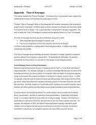
Unconstrained Optimization (2)F(X)BDACE●By calculus:XIf F(X) continuous, analytic:Condition for maxima and minima∂F(X) / ∂X i = 0 ∀ iEngineering Systems Analysis for Design Richard de Neufville, Joel Clark, and Frank R. FieldMassachusetts Institute of Technology Constrained Optimization Slide 3 of 23Unconstrained Optimization (3)●Secondary conditions:∂ 2 F(X) / ∂X2i < 0 = > Max (B,D)∂ 2 F(X) / ∂X2i > 0 = > Min (A,C,E)These define whether point of no changein Z is a maximum or a minimumEngineering Systems Analysis for Design Richard de Neufville, Joel Clark, and Frank R. FieldMassachusetts Institute of Technology Constrained Optimization Slide 4 of 23Page 2

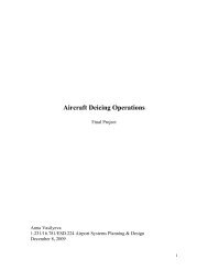
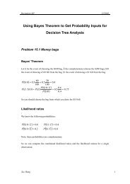
Unconstrained Optimization (4)●Example: Housing insulationF(x) = K 1 / x + K 2 xTotal Cost = Fuel cost + Insulation costx = Thickness of insulation∂F(x) / ∂x = 0 = -K 1 / x 2 + K 2=> x* = {K 1 / K 2 } 1/2(starred quantities are optimal)Engineering Systems Analysis for Design Richard de Neufville, Joel Clark, and Frank R. FieldMassachusetts Institute of Technology Constrained Optimization Slide 5 of 23Unconstrained Optimization (5)● K 1 = 500 K 2 = 24 X* = 4.56Optimizing Cost ExampleCost60050040030020010001 3 5 7 9 11Inches of InsulationFuelInsulationTotalEngineering Systems Analysis for Design Richard de Neufville, Joel Clark, and Frank R. FieldMassachusetts Institute of Technology Constrained Optimization Slide 6 of 23Page 3

●●Constained Optimization“Constrained Optimization” involves theoptimization of a process subject toconstraintsConstraints have two basic types— Equality Constraints -- some factors have toequal constraints— Inequality Constraints -- some factors have tobe less less than or greater than theconstraints (these are “upper” and “lower”boundsEngineering Systems Analysis for Design Richard de Neufville, Joel Clark, and Frank R. FieldMassachusetts Institute of Technology Constrained Optimization Slide 7 of 23Equality Constraints●●●Example: Best use of budgetMaximize: Output = Z(X) = a o x 1a1x 2a2Subject to (s.t.):Total costs = Budget = p 1 x 1 + p 2 x 2Z(x)Z*BudgetNote: ∂Z(X) / ∂X ≠ 0 at optimumXEngineering Systems Analysis for Design Richard de Neufville, Joel Clark, and Frank R. FieldMassachusetts Institute of Technology Constrained Optimization Slide 8 of 23Page 4

●ApproachConstrained OptimizationTo solve situations of increasingcomplexity, (for example, those withequality, inequality constraints) ...●Transform more difficult situation intoone we know how to deal withIn this case, transform optimization of a“constrained” situation to optimization of“unconstrained” situationEngineering Systems Analysis for Design Richard de Neufville, Joel Clark, and Frank R. FieldMassachusetts Institute of Technology Constrained Optimization Slide 9 of 23●●●Lagrangean Method (1)Transforms equality constraints intounconstrained problemStart with:Opt: F(x)s.t.: g j (x) = b j => g j (x) - b j = 0Get to:L = F(x) - Σ j λ j [g j (x) - b j ]λj = Lagrangean multipliers (lambdas) -- theseare unknown quantities for which we must solveNote: [g j (x) - b j ] = 0 by definition, thusoptimum for F(x) = optimum for LEngineering Systems Analysis for Design Richard de Neufville, Joel Clark, and Frank R. FieldMassachusetts Institute of Technology Constrained Optimization Slide 10 of 23Page 5

Lagrangean Method (2)● To optimize L:●∂L / ∂x i = 0 ∀ i∂L / ∂λ j = 0 ∀ iExample:Opt: F(x) = 6x 1 x 2s.t.: g(x) = 3x 1 + 4x 2 = 18L = 6x 1 x 2 - λ(3x 1 + 4x 2 - 18)∂L / ∂x 1 = 6x 2 - 3λ = 0∂L / ∂x 2 = 6x 1 - 4λ = 0∂L / ∂λ i = 3x 1 + 4x 2 -18 = 0Engineering Systems Analysis for Design Richard de Neufville, Joel Clark, and Frank R. FieldMassachusetts Institute of Technology Constrained Optimization Slide 11 of 23●Lagrangean Method (3)Solving as unconstrained problem:∂L / ∂x 1 = 6x 2 - 3λ = 0∂L / ∂x 2 = 6x 1 - 4λ = 0∂L / ∂λ i = 3x 1 + 4x 2 -18 = 0● so that: λ = 2x 2 = 1.5x 1x 2 = 0.75x 13x 1 + 3x 1 - 18 = 0● x 1 * = 18/3 = 6 x 2 * = 18/8 = 2.25 λ* = 4.5● F(x)* = 40.5Engineering Systems Analysis for Design Richard de Neufville, Joel Clark, and Frank R. FieldMassachusetts Institute of Technology Constrained Optimization Slide 12 of 23Page 6

●●●●Shadow PricesShadow Price is the Rate of change ofobjective function per unit change ofconstraint= ∂F(x) / ∂b jThis is meaning of Lagrangean multiplierSP j = ∂F(x)*/ ∂b j = λ j— Naturally, this is an instantaneous rateThe shadow price is extremely importantfor system designIt defines value of changing constraintsEngineering Systems Analysis for Design Richard de Neufville, Joel Clark, and Frank R. FieldMassachusetts Institute of Technology Constrained Optimization Slide 13 of 23●●Shadow Prices (2)Let’s see how this works in example, bychanging constraint by 0.1 units:Opt: F(x) = 6x 1 x 2s.t.: g(x) = 3x 1 + 4x 2 = 18.1The optimum values of the variables arex 1 * = (18.1)/6 x 2 * = (18.1)/8● Thus F(x)* = 6(18.1/6)(18.1/8) = 40.95∆F(x) = 40.95 - 40.5 = 0.45 = λ* (0.1)Engineering Systems Analysis for Design Richard de Neufville, Joel Clark, and Frank R. FieldMassachusetts Institute of Technology Constrained Optimization Slide 14 of 23Page 7

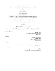
●Inequality ConstraintsExample: Housing insulationMin: Costs = K 1 / x + K 2 xs.t.: x ≥ 8 (minimum thickness)Optimizing Cost ExampleCost60050040030020010001 3 5 7 9 11Inches of InsulationFuelInsulationTotalEngineering Systems Analysis for Design Richard de Neufville, Joel Clark, and Frank R. FieldMassachusetts Institute of Technology Constrained Optimization Slide 15 of 23●Inequality Constraints (2)Approach: Transform inequalities intoequalities, then proceed as before●Again, introduce new variable -- the“Slack” variable that defines “slack” ordistance between constraint and amountused●The resulting equations are known as the“Kuhn-Tucker conditions”Engineering Systems Analysis for Design Richard de Neufville, Joel Clark, and Frank R. FieldMassachusetts Institute of Technology Constrained Optimization Slide 16 of 23Page 8

●●Inequality Constraints -- insertion ofslack variables in LagrangeanA “slack variable”, s j , for each inequalityg j (x) ≤ b j => g j (x) + s2 j = b jg j (x) ≥ b j => g j (x) - s2 j = b jThese are “squared” to be positive●start from:opt: F(x)s.t.: g j (x) ≤ b j●get to:L = F(x) - Σ j λ j [g j (x) + s j2- b j ]Engineering Systems Analysis for Design Richard de Neufville, Joel Clark, and Frank R. FieldMassachusetts Institute of Technology Constrained Optimization Slide 17 of 23Inequality Constraints --Complementary Slackness Conditions●The optimality conditions are:∂L / ∂x i = 0∂L / ∂λ j = 0plus: ∂L / ∂s j = 2s j λ j = 0●These new equations imply:s j = 0orλ j ≠ 0s j ≠ 0 λ j = 0They are the “complementary slackness”conditions. Either slack or lambda =0 ∀ iEngineering Systems Analysis for Design Richard de Neufville, Joel Clark, and Frank R. FieldMassachusetts Institute of Technology Constrained Optimization Slide 18 of 23Page 9

●Interpretation of ComplementarySlackness ConditionsInterpretation:● If there is slack on b j ,(i.e. more than enough of it)=> No value to objective functionto having more: λ j = ∂F(x) / ∂b j = 0●If λ j ≠ 0, then all available b j used=> s j = 0Engineering Systems Analysis for Design Richard de Neufville, Joel Clark, and Frank R. FieldMassachusetts Institute of Technology Constrained Optimization Slide 19 of 23●Application to ExampleMin: Costs = K 1 / x + K 2 xs.t.: x ≥ 8 (minimum thickness)● L = K 1 /x + K 2 x - λ[x - s 2 - b]● L = 500/x + 24x - λ[x - s 2 - 8]● 500/x 2 + 24 - λ = 0 2 λs = 0 x - s 2 = 8●●If s = 0, x = 8, λ = 31.8 (at that point)Max = 254.5Therefore, worth relaxing (in this case,lowering) constraint to get maximum● x * = 4.56 Optimum = 221Engineering Systems Analysis for Design Richard de Neufville, Joel Clark, and Frank R. FieldMassachusetts Institute of Technology Constrained Optimization Slide 20 of 23Page 10

Unconstrained Optimization (5)● K 1 = 500 K 2 = 24 X* = 4.56Optimizing Cost ExampleCost60050040030020010001 3 5 7 9 11Inches of InsulationFuelInsulationTotalEngineering Systems Analysis for Design Richard de Neufville, Joel Clark, and Frank R. FieldMassachusetts Institute of Technology Constrained Optimization Slide 21 of 23●Another application to ExampleMin: Costs = K 1 / x + K 2 xs.t.: x ≥ 4 (NEW MINIMUM)● L = K 1 /x + K 2 x - λ[x + s 2 - b]● L = 500/x + 24x - λ[x + s 2 - 4]● 500/x 2 + 24 - λ = 0 2 λs = 0 x - s 2 = 4● If λ = 0, x = 4.56, slack, s 2 = 1.56Optimum = 221●not worth changing constraintEngineering Systems Analysis for Design Richard de Neufville, Joel Clark, and Frank R. FieldMassachusetts Institute of Technology Constrained Optimization Slide 22 of 23Page 11

Summary of Presentation●Important mathematical approaches— Lagreangeans— Kuhn- Tucker Conditions●Important Concept: Shadow Prices●THESE ANALYSES GUIDE DESIGNERSTO CHALLENGE CONSTRAINTSEngineering Systems Analysis for Design Richard de Neufville, Joel Clark, and Frank R. FieldMassachusetts Institute of Technology Constrained Optimization Slide 23 of 23Page 12