The Onsager Equation for Corpora - Department of Mathematics

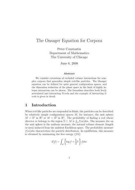
where b is a nonnegative parameter, representing a combination of inversetemperature and intensity of interaction, and∫U(m) = u(m, p)f(p)dpMis a potential computed from an interaction kernel u(m, p). The physicalmodeling is reflected in the choice of kernel. Only two effects are taken intoaccount in the free energy: an entropic effect, representing thermal fluctuationof the particles, and a quadratic mean field effect representing excludedvolume interactions between particles. The description of the problem iscompleted by specifying the configuration space M, the uniform measure dmand the interaction kernel u. Once these are determined we may ask questions,such as: do minima of the free energy exist, how many such minimaexist, what happens to them as the parameter b varies from b = 0 to infinity.In the case of more complicated corpora, the configuration space M canbe rather complicated. We use the word “corpus” to refer to a body thathas finitely many degrees of freedom, such as an assembly of articulatedrods, or rods connected to balls of different sizes and with different motionconstraints between the parts. The collection of all corpora of a particularproblem is the configuration space. It is useful to phrase the equilibrium andkinetic problems broadly, in quite general configuration spaces. We consider ametric space M, with distance d, and assume we are given a Borel probabilitymeasure µ on M. This probability measure corresponds to the normalizeduniform distribution of corpora m ∈ M, and M is the configuration space.For absolutely continuous probability Borel measures ν

Because ∫ Ufdµ = ∫ ∫u(x, y)f(x)f(y)dµ(x)dµ(y), there is no loss ofM M Mgenerality by assuming that u(x, y) is symmetric, as only the symmetric part1(u(x, y) + u(y, x)) contributes to the free energy. Critical points of the free2energy obeyδEδf = 0which leads to Onsager’s equation:f = Z −1 e −bU (2)Indeed, this follows taking the Gateaux derivative (i.e. the first variation) ofE in a direction h, i.e.ddt E[f + th] | t=0 = 0,with arbitrary h, subject only to ∫ hdµ = 0 in order to respect ∫ (f +M Mth)dµ = 1. A simple calculation, using the fact that u(x, y) is symmetric inx, y leads to ∫ (log f + bU)hdµ = 0 for all h. This implies that log f + bU isMconstant µ-almost everywhere. Because u is Lipschitz continuous, it is easyto see that the solutions of (2) are Lipschitz continuous, positive and nevervanish.The kernel u gives the rule to construct the potential U associated to theparticle distribution ν = fdµ; in examples this is computed from physicsand it instructs the particles to conform to each other. As b → ∞ thereare phase transitions. In the abstract case where we have a distance d wemay consider general u(x, y) = Φ(d(x, y), x, y) and the simplest examplesare u(x, y) = d(x, y) p with p = 1, 2 or u(x, y) = −e − d2 (x,y)l 2 . The interactionpotential u(x, y) should have a minimum at x = y.2 RodsThe simplest example of single rods has M = S 1 . The Onsager kernel isu(θ 1 , θ 2 ) = | sin(θ 1 − θ 2 )|, and the Maier-Saupe kernel isu(θ 1 , θ 2 ) = − cos 2 (θ 1 − θ 2 ).Kernels are defined up to addition of constants, so the Maier-Saupe kernelcan be taken as u(θ 1 , θ 2 ) = − cos(2(θ 1−θ 2 ))2.3

Throughout this paper we will use the notation Kf = −U[f] = −U toemphasize the linear dependence of U on f. (The minus sign is a conventionwe maintain to be consistent with previously published literature.)In the Maier-Saupe potential case, Kf projects f on the eigenspace ofthe Laplace-Beltrami operator corresponding to eigenvalue 4. If the functionf is written asf(θ) = 12π + 1 ∞∑y j cos(2jθ) (3)πthen Maier-Saupe potential isj=1Kf = 1 2 y 1 cos(2θ). (4)The solutions of the Onsager equation in that case are of the formwithand in Fourier representationg(r) = (Z(r)) −1 e r cos(2θ) (5)Z(r) =∫ 2πg(r)(θ) = 12π + 1 π0e r cos(2θ) dθ (6)∞∑g j (r) cos(2jθ) (7)Onsager’s equation is equivalent to the implicit transcendental equationj=1g 1 (r) = 2rb . (8)If b ≤ 4 this equation has one solution, namely r = 0. If b > 4 there isexactly one more solution for r > 0 at r = r(b). There is exactly one solutionfor r < 0, at r = −r(b) corresponding to a rotation of π of the solution with2r > 0. It is known also that g 0 (r) = 1 for all r,g j (r) > 0, g j+1 (r) < g j (r), j ≥ 1, r > 0. (9)If r = r(b) is determined by (8), theng 2 (r(b)) = 1 − 4 b ,4

there are recursion relations to compute all g j (r), anddbdr = b2 ( )g22r 1 − g 2 > 0 (10)holds for the inverse function, b(r). This is an increasing unbounded functionfor b > 4. The stability of the solution g(r) also follows from the inequalityg 2 1 − g 2 > 0. Both the inequality and the stability are not obvious. The limitof zero temperature is a delta function:lim g (r(b))(θ)dθ = δ 0 . (11)b→∞The choice of θ = 0 is dictated by the symmetry θ ↦→ −θ that we imposed.Otherwise, we obtain any delta function on the circle. The case of S 2 withMaier-Saupe potential is similar. The potential projects on the eigenspace ofeigenvalue 6 of the Laplace-Beltrami operator on the sphere. Two implicittranscendental equations determine the solution. There is a finite temperaturephase transition and the zero temperature limits are delta functions onpoints or geodesics.3 KineticsThe kinetic description of rod-like particles ([9]) can be naturally generalizedwhen the configuration space M is a Riemannian manifold. When M isRiemannian manifold, the kinetic equations are∂ t f = ∆ g f − bdiv g (f∇ g (Kf)) (12)with ∆ g , div g , ∇ g Laplace-Beltrami, divergence and gradient in M, Kf givenby∫Kf = − u(m, p)f(p)dµ(p) (13)Mand the uniform measure dµ is the Riemannian volume element. Note thatthe equation can be written as∂ t f = div g (f∇ g (log f − bKf))The solutions are smooth, positive and normalized so they have unit integral.The free energy∫E ={f log f − b }2 fKf dµ (14)5

is a Lyapunov functional:∫ddt E = − f |∇ g (log f − bKf)| 2 dµ(p)MIf M is connected, the only possible steady solutions are solutions of Onsager’sequationf = Z −1 e bKf . (15)The dynamical system is dissipative: the solutions are bounded after aninitial transient time. The bounds, in very strong norms, are independent ofthe initial data. The global attractor is compact, finite dimensional and isformed with solutions of Onsager’s equations and their unstable manifolds.In the case of M = S 1 with Maier-Saupe potential, the kinetic equations aregiven by the sequence of ODEsddt y j = −4j 2 y j + bjy 1 (y j−1 − y j+1 ) . (16)The equations on S 2 are more complicated. Some of the results concerningequilibria and kinetics for the Maier-Saupe potential can be found in [1] -[4],[6], [7], [10] -[14] and [19]. Recently it was shown that the system has inertialmanifolds in both S 1 and S 2 ([17]-[18]).4 Freely articulated corporaWe consider corpora made of N articulated rods that are allowed to rotatefreely. The configuration space is ˜M = S n × · · · × S n with n = 1 or 2. Thepotential is a sum of binary interactionsv(p 1 , q 1 , p 1 , q 2 , . . . p N , q N ) =N∑u j (p j , q j ). (17)j=1The uniform measure µ on ˜M is the product measure. In this situation, thecorresponding solution of the Onsager equation is a product measureν(dp 1 . . . dp N ) = Π N j=1Z −1j e −bU j(p j ) dp j (18)where each Z −1j e −bU j(p j ) is a solution of Onsager’s equation in the j component,and everything can be reduced to the study of individual rods. This6

∫ 2πZ = e −b sin2 (θ)+2bz sin θ−bγ dθ0The solution is f(p 1 , p 2 ) = g(p 1 − p 2 ). Note that g does not depend on γ.Let thens(θ, z) = sin θ − z,and let∫ 2πs(θ, z)e −bs2 (θ,z) dθ0[s](b, z) = ∫ 2π.e0 −bs2 (θ,z)dθThe Onsager equation is equivalent to[s](b, z) = 0. (19)This determines z, which in turn determines g, f. Note that z = 0 always asolution that yieldsf 0 (p 1 , p 2 ) = Z −1 e −b sin2 (p 1 −p 2 ) .As b → ∞ this solution tends to δ((p 1 − p 2 ) modπ), a degenerated two-rod.Consider nowwith τ = b −1 . Note thatso (19) is equivalent toλ(z, τ) = b 1 2∫ 2π0e −b(sin θ−z)2 dθ[s](τ −1 , z) = 1 ∂ z λ2b λ∂ z λ = 0. (20)Note also that λ solves a linear heat equation with temperature as time:∂ τ λ = 1 4 ∂2 zλThe function λ is even in z, so it is enough to study it on [0, 1]. The “initialvalue” obeys, for any z ∈ [0, 1),lim λ(z, τ) = 2√ 1π √τ→0 1 − z29

for all x ∈ M, and all r sufficiently small. Here B(x, r) is the ball centeredat x ∈ M and of radius r in the metric d. This assumption says thatall balls are charged at least a small positive amount. Note that if M isany compact Riemannian manifold of dimension n and µ is the Riemannianvolume element, then the condition (21) is automatically satisfied, because r nis much larger, for small r, than the right hand side of (21). The interactionkernel we consider is a function of the distance, u(d(x, y)), so∫U(x) = u(d(x, y))f(y)dµ(y). (22)MWe assume that u is non-negative, bounded and Lipschitz continuous, i.e.there exist positive constants C and L so thatandhold for all d, d 1 , d 2 ≥ 0. We assume also that0 ≤ u(d) ≤ C (23)|u(d 1 ) − u(d 2 )| ≤ L |d 1 − d 2 | (24)u(0) = 0. (25)As we mentioned before, the interaction kernels are defined up to additiveconstants: if we add c to the interaction kernel, then the potential is changedby the same amount c and the free energy is changed by adding bc ; its critical2points, and in particular its minima are unchanged. Let us take a ball of Bof radius r, set χ = µ(B) −1 1 B the normalized indicator function of B, andcomputeE[χ] = log(µ(B) −1 ) + b ∫ ∫2 µ(B)−2 u(d(x, y))dµ(x)dµ(y)We obtain, using (21, 23, 24) that( ) k ( )1 1E[χ] ≤ + log + bLrr cwhich implies, by choosing r = b −1 , thatBBinff E[f] ≤ bk + C 111

holds for large b with some constant C 1 . This means that uniform measure,whose energy is linear in b,E[1] = b ∫ ∫u(d(x, y))dµ(x)dµ(y)2MMdoes not achieve the minimum of energy for large b. On the other hand,for may examples, the uniform measure is a solution of Onsager’s equation.Indeed, if T is a µ measure preserving isometry of M, then the potentialassociated to the uniform measure µ, U[1] = −K1, is invariant under rightcomposition with T , i.e.,U(T x) = U(x)holds for all x ∈ M and all measure preserving isometries. If measure preservingisometries act transitively, i.e., for any x, y ∈ M there exists T ameasure preserving isometry that maps x to y, y = T x then, U = −K(1) isa constant. This implies that the uniform measure is a solution of Onsager’sequation. This is the case for many homogeneous spaces. The combination ofthese two very simple observations leads to the conclusion that a phase transitionoccurs, whenever the homogeneous measure is a solution of Onsager’sequation, the condition (21) holds and the interaction kernel is a normalizedLipschitz function of distance. That simply means that, while for b = 0 obviouslythe only solution of Onsager’s equation is the homogeneous measure,and while this continues to be a solution for b > 0, at large enough b thereexist other solutions as well, in quite great generality.Now we describe a general tendency of solutions to concentrate. Letdν = fdµ be any probability measure absolutely continuous with respect toµ and let U be the potential associated to it via (22). Then, in view of theproperty (23) we have0 ≤ U(x) ≤ C (26)and from (24) and the triangle inequality we deduce that|U(x) − U(y)| ≤ Ld(x, y) (27)so that the potentials associated to any probability fdµ are non-negative,uniformly bounded and Lipschitz continuous.Theorem 1 Let M be a compact metric space with distance d. Let µ be aBorel probability measure on M that satisfies (21). Let u satisfy (23,24).Then:12

(A) For any b > 0 there exists a solution g that minimizes the enery:E[g] =minf>0, R E[f]M fdµ=1The function g solves the Onsager equationwithandg(x) = (Z(b)) −1 e −bU(x)∫Z(b) =∫U(x) =MMe −bU(x) dµ(x)u(d(x, y))g(y)dµ(y)The function g is normalized ∫ gdµ = 1, strictly positive and Lipschitz continuous.(B) Let b n → ∞ and let dν n = g n dµ be a sequence of solutions of Onsagerequations corresponding to b n . By passing to a subsequence we may assumethat the sequence converges weakly to a probability measure ν = lim n ν n .There exists a non-negative Lipschitz continuous function U ∞ (x) on M suchthat ν is concentrated on the setΣ = {x ∈ M | U ∞ (x) = min y∈M U ∞ (y)}Thus, for any continuous function φ supported in the open set M \ Σ,∫φ(x)g n (x)dµ = 0limn→∞MProof. For the proof of (A) we fix b > 0 and note that E[f] is bounded belowuniformly for all f > 0, ∫ fdµ = 1. We take then a minimizing sequenceMf j ,a = inff>0; R E[f] = lim E[f j ].M fdµ=1 j→∞Without loss of generality, by passing to a subsequence and relabelling, wemay assume that the measures f j dµ converge weakly to a measure dν. Using(26, 27) and the Arzela-Ascoli theorem, we may pass to a subsequence, whichwe relabel again f j , so that U j converge uniformly to a non-negative Lipschitzcontinuous function U. Then it follows that∫U(x) = u(d(x, y))dν(y)M13

holds and∫∫lim U j f j dµ = Udν.j→∞MMBecause E[f j ] is a convergent sequence of numbers, it follows that∫limj→∞Mf j log f j dµexists. In particular, the above integrals are bounded uniformly. It thenfollows that dν is absolutely continuous i.e., dν = gdµ, with g ≥ 0, g ∈L 1 (dµ). Indeed, the sequence f j dµ is uniformly absolutely continuous. Thisfollows from the convexity of the function y log y and the Jensen inequality∫(µ(A)) −1 f log fdµ ≥ m log mwhere m = µ(A) ∫ −1 fdµ. Then we haveAAm log m ≤ C/µ(A)with a fixed constant C > 0, uniformly for all f = f j and any A. Let uschoose R so that R log R = C/µ(A). If we denote by I = ∫ fdµ, then eitherAm ≤ R, or, if not, then m log R ≤ C/µ(A). In either case the inequalitiesimplyI ≤ C/ log(R)and as µ(A) → 0, R → ∞. This inequality signifies∫f n dµ ≤ δ(µ(A))Awith lim x→0 δ(x) = 0 and δ(x) independent of n. This implies that ν is absolutelycontinuous, ν = gdµ with 0 ≤ g ∈ L 1 (dµ). The weak convergencetested on the function 1 implies that ∫ gdµ = 1. In general, weak convergenceof measures is not enough to show lower semicontinuity of nonlinearintegrals or almost everywhere convergence. We claim however that in factthe convergence f n → g takes place strongly in L 1 (dµ):∫limn→∞M|f n (x) − g(x)|dµ(x) = 0.14

In order to prove this we prove that f n is a Cauchy sequence in L 1 (dµ). Wetake ɛ > 0 and choose N large enough so thatand∫∣Msup |U n (x) − U(x)| ≤ ɛ2x∈M10b ,U(x)(f n (x) − f m (x))dµ∣ ≤ ɛ210bE[f n ] ≤ a + ɛ216hold for n, m ≥ N. Let s(x) = 1(f 2 n(x) + f m (x)). Then ∫ sdµ = 1, s > 0,Msoa ≤ E[s].Therefore12 {E(f n) + E(f m )} − E[s] ≤ ɛ216 .On the other hand,∫ { 12 [f n log f n + f m log f m ] − s log s}dµ ≤ 1 2 {E(f n) + E(f m )} − E[s] + ɛ216soM∫M{ 12 [f n log f n + f m log f m ] − s log s}dµ ≤ ɛ2 8 .Denote χ = fn−fmf n+f mand note that −1 ≤ χ ≤ 1 holds µ - a.e. Also, elementarycalculation show that{ 12 [f n log f n + f m log f m ] − s log s}= s 2 G(χ)holds with( 1 + χG(χ) = log(1 − χ 2 ) + χ log1 − χ(Note that G is even on (−1, 1), that G ′ (χ) = logand G ′′ (χ) = 21−χ 2≥ 2 on (−1, 1). Consequently,0 ≤ χ 2 ≤ G(χ)151+χ1−χ).), G(0) = G ′ (0) = 0

holds for −1 ≤ χ ≤ 1. It follows that we have∫(f n − f m ) 2dµ ≤ ɛ2f n + f m 2MBut, writing |f n − f m | = √ |ff n + f n−f m|m√ fn+fmand using the Schwartz inequalitywe deduce∫|f n − f m |dµ ≤ ɛ.MTherefore the sequence f n is Cauchy in L 1 (dµ). This proves that the weaklimit f n dµ → gdµ is actually strong f n → g in L 1 (dµ). By passing to asubsequence if necessary, we may assume also that f n → g holds also µ- a.e.Then, from Fatou’s Lemma∫∫g log gdµ ≤ lim f j log f j dµ.j→∞This implies thatME[g] = a.The fact that g solves the Onsager equation follows by taking the Gateauxderivative, and thusg = Z −1 e −bUwith Z = ∫ M e−bU dµ. Because U is bounded it follows that g never vanishesand because U is Lipschitz, so is g.The proof of (B). Let b n → ∞ and let us take a subsequence so that g n dµconverges weakly to dν. As above, because of (26, 27) and the Arzela-Ascolitheorem, we may pass to a subsequence, which we relabel again g n , so thatU n converge uniformly to a non-negative Lipschitz continuous function U ∞ .Let x n be a point where U n (x) attains its minimum U n (x n ) = min x∈M U n (x).By passing again to a subsequence we may assume that x n converge to somepoint x. It follows that that U ∞ (x) = min m∈M U ∞ (m) = α. Let φ be acontinuous function in M compactly supported in M \ Σ where Σ = {m ∈M | U ∞ (m) = α}. There exists ɛ > 0 so that, for every m in the support ofφ, U ∞ (m) ≥ α + 4ɛ. Let us take N so large that sup M |U ∞ (m) − U n (m)| ≤ ɛfor n ≥ N and d(x n , x) ≤ ɛ Denote α L nthe minimum of U n . It follows that|α n − α| ≤ 2ɛ and U n (m) ≥ α n + ɛ on the support of φ. On the other hand,we have∫∫Z n (b n ) ≥ e −bnUn(z) dµ(z) ≥ e −bnαn e −bnLd(z,xn) dµ(z),B(x n, 1bn ) B(x n, 1bn )16

and using (21) we getTherefore, on the support of φ we haveZ n (b n ) ≥ e −L ce −bk n e−b nα n(28)g n (m) = (Z n (b)) −1 e −bnUn(m) ≤ e L c −1 e bk n eb nα ne −bn(αn+ɛ)and consequently∫∫∣ φ(m)g n (m)dµ(m)∣ ≤ eL c −1 e bk n e−b nɛMholds, and therefore, as k < 1 we have∫φg n dµ = 0.7 Conclusionslimn→∞MM|φ(m)|dµ(m) (29)The generalization of excluded volume interactions, from simple rod-like particlesto complicated corpora leads to a “simple” equation (the Onsager equation)in “complicated” spaces. The examples of single rods, and articulatedtwo-rods show significant complexity reduction. The complexity reduction,once the problem is phrased correctly, is expected to be generic. The zerotemperature or high intensity limit of probability distributions of corporaconcentrates on the minima of certain Lipschitz functions, in general.8 AcknowledgmentsWork partially supported by NSF-DMS grant 0504213. I thank A. Zlatosand B. Farb for fruitful conversations.References[1] P. Constantin, Nonlinear Fokker-Planck Navier-Stokes Systems, Commun.Math. Sci. 3 (2005), 531-544.17

[2] P. Constantin, Smoluchowski Navier Stokes Systems, ContemporaryMathematics 429, G-Q Chen, E. Hsu, M. Pinsky editors, AMS, Providence(2007), 85 - 109.[3] P. Constantin, I. Kevrekidis, E. S. Titi, Remarks on a SmoluchowskiEquations, Discrete and Continuous Dyn. Syst, 11 (2004) 101-112.[4] P. Constantin, I. Kevrekidis, E.S. Titi, Asymptotic states of a Smoluchowskiequation, ARMA 174 (2004), 365-384.[5] P. Constantin, Ch. Fefferman, E.S. Titi, Global Regularity for Smoluchowskiequations coupled to fluids, article in preparation.[6] P. Constantin, E.S. Titi, J. Vukadinovic, Dissipativity and GevreyRegularityof a Smoluchowski Equation, Indiana U. Math J., 54 (2005),949-969.[7] P. Constantin, J. Vukadinovic, Note on the number of steady states fora 2D Smoluchowski equation, Nonlinearity 18 (2005) 441-443.[8] P. Constantin, A. Zlatos, The Onsager equation for articulated rods inspace, in preparation.[9] M. Doi, S.F. Edwards, The Theory of Polymer Dynamics, Oxford UniversityPress, Oxford 1988.[10] I. Fatkullin, V. Slastikov, A note on the Onsager model of nematic phasetransitions, Commun. Math. Sciences. 3 (2005), 21-.[11] H. Zhou, H. Wang, M.G. Forest, Q. Wang, A new proof on axisymmetricequilibria of a three-dimensional Smoluchowski equation, Nonlinearity 18(2005) 2815-2825.[12] G. Forest, Q. Wang, R. Zhou, The weak shear phase diagram for nematicpolymers, Rheologica Acta, 43 (2004), 17-37.[13] C. Luo, H. Zhang, P-W. Zhang, The structure of the equilibrium solutionsof one dimensional Doi equation, Nonlinearity 18 (2005), 379-389.[14] H. Liu, H. Zhang, P-W Zhang, Axial symmetry and classification ofstationary solutions of Doi-Onsager Equation on the sphere with Maier-Saupe potential. Comm. Math. Sci. 3 (2005), 201-218.18

[15] L. Onsager, The effects of shape on the interaction of colloidal particles,Ann. N.Y. Acad. Sci 51 (1949), 627-659.[16] F. Otto, A. Tzavaras, Continuity of velocity gradients in suspensions ofrod-like molecules, SFB Preprint 147 (2004).[17] J. Vukadinovic, Inertial Manifolds for a Smoluchowski equation on acircle, preprint (2008)[18] J. Vukadinovic, Inertial Manifolds for a Smoluchowski equation on theunit sphere, preprint (2008).[19] A. Zarnescu, Thesis, the University of Chicago, (2006).19