Decimation and Interpolation

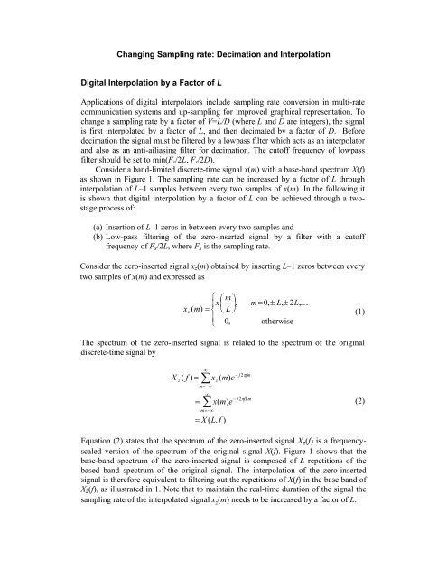
Changing Sampling rate: Decimation and InterpolationDigital Interpolation by a Factor of LApplications of digital interpolators include sampling rate conversion in multi-ratecommunication systems and up-sampling for improved graphical representation. Tochange a sampling rate by a factor of V=L/D (where L and D are integers), the signalis first interpolated by a factor of L, and then decimated by a factor of D. Beforedecimation the signal must be filtered by a lowpass filter which acts as an interpolatorand also as an anti-ailiasing filter for decimation. The cutoff frequency of lowpassfilter should be set to min(F s /2L, F s /2D).Consider a band-limited discrete-time signal x(m) with a base-band spectrum X(f)as shown in Figure 1. The sampling rate can be increased by a factor of L throughinterpolation of L–1 samples between every two samples of x(m). In the following itis shown that digital interpolation by a factor of L can be achieved through a twostageprocess of:(a) Insertion of L–1 zeros in between every two samples and(b) Low-pass filtering of the zero-inserted signal by a filter with a cutofffrequency of F s /2L, where F s is the sampling rate.Consider the zero-inserted signal x z (m) obtained by inserting L–1 zeros between everytwo samples of x(m) and expressed as⎧ ⎛ m ⎞⎪x⎜⎟,m = 0, ± L,± 2L,Kx z( m)= ⎨ ⎝ L ⎠(1)⎪⎩ 0, otherwiseThe spectrum of the zero-inserted signal is related to the spectrum of the originaldiscrete-time signal byXz( f ) =zm=−∞=∞∑∞∑m=−∞x ( m)ex(m)e= X ( L.f )− j2πfm− j2πfLm(2)Equation (2) states that the spectrum of the zero-inserted signal X z (f) is a frequencyscaledversion of the spectrum of the original signal X(f). Figure 1 shows that thebase-band spectrum of the zero-inserted signal is composed of L repetitions of thebased band spectrum of the original signal. The interpolation of the zero-insertedsignal is therefore equivalent to filtering out the repetitions of X(f) in the base band ofX z (f), as illustrated in 1. Note that to maintain the real-time duration of the signal thesampling rate of the interpolated signal x z (m) needs to be increased by a factor of L.

Interpolation Using DFTTaking the DFT of N samples of zero-inserted signal we haveXz( k)=NL−1m=0=∑N∑m=0= X ( k)x ( m)ezx(m)e2π− j mkNL2π− j mkNNLk=0,1,, …, NL-1 (3)Note from this equation that within a frequency interval of to 2π or (0 to F S Hz) thereare L repetition of the spectrum of X(k), this is because stretching the signal by afactor of L shrinks its spectrum by a factor of 1/L.(a)(b)(c)(d)(e)Figure(1) - (a) Original signal, (b) zero-insetred signal, (c) spectrum of original signal,(d) spectrum of zero-inserted signal, (e) interpolated signal

Digital Decimation by a Factor of LConsider a band-limited discrete-time signal x(m) with a base-band spectrumX(f). The sampling rate can be decreased by a factor of L through discarding of L–1samples for every L samples of x(m). In the following it is shown that digitaldecimation by a factor of L can be achieved through a two-stage process of:(a) Low-pass filtering of the zero-inserted signal by a filter with a cutofffrequency of F s /2L, where F s is the sampling rate. This is the anti-alisaingprocess.(b) Discarding of L–1 samples for every L samples.Mathematical model of decimation. Consider a resampled signal x r (m) expressed asthe product of the orginal sample x(m) and the resampling pulse train p(m) as( Lm),⎧ = ± ±= = ∑ ∞ x m 0, 1, 2, Kxr( m)x(m).p(m)x(k)δ ( k − Lm)= ⎨k = −∞⎩ 0, otherwise(4)where the pulse train p(m) is given by∑ ∞k = −∞p ( m)= δ ( k − Lm)⇔P(f ) =∑ ∞k = −∞⎛δ ⎜ f⎝− kFsL⎞⎟⎠(5)Note as the distance between pulses increase by a factor of L the distance betweentheir frequency components shrink by a factor of 1/L.From the Fourier properties, the spectrum of a resampled signal is the convolution ofthe spectra of the x(m) and p(m)X ( f ) =r∑ ∞k = −∞⎛ FsX ⎜ f + k⎝ LThe down-sampled signal can be obtained from the resampled signal asx ( m)x ( mL)d=r⎞⎟⎠(6)(7)

SignalRe-sampling (down-sampling) functionδ(0) δ(L) δ(2L) δ(3L) δ(4L) …Figure2 Resampling process.The spectrum of the decimated signal can be related to the spectrum of the resampleddiscrete-time signal as followsXd( f ) ===N −1∑m=0∞∑x ( m)edrm=−∞∞∑rm=−∞x ( m)e− j 2πfmx ( mL)ef− j2πmLLf− j2πmL= Xr( f / L)(8)Note that in developing the third line of Eq(8) from the second line we used the factthat inbetween every two signal samples of x r (m) there are L-1 zeros.Figure 3 (a) Decimated signal and (b) its spectrum.