Reduced point mass or multipole base functions. - Niels Bohr Institutet

Reduced point mass or multipole base functions.C.C.Tscherning, M.Veicherts, 1 M.Herceg 2 ,1 Niels Bohr Institute, University of Copenhagen, Denmark.2 DTU Space, Denmark.Juliane Maries Vej 30, DK 2100 Copenhagen Oe, Denmark.Abstract: Point-mass functions or multipole base-functions are harmonicfunctions, which may be used to represent the (anomalous) gravity potential (T)globally or locally. The functions may be expressed by closed expressions or assums of Legendre series. In both cases at least the two first terms must be removedsince they are not present in T. For local applications the effect of a global gravitymodel is generally removed (and later restored). Then more terms need to beremoved or substituted by terms similar to error-degree variances. We have donesome calculations to illustrate the effect of reducing the point mass or multipolefunctions, i.e. showing how the first zero-crossing as a function of sphericaldistance comes closer to zero when more terms are removed.1. Introduction.Linear combinations of point mass functions or mass multipoles have been usedfor the representation of the global (W) or regional anomalous gravity potential, T,see e.g. Balmino (1974), Hauck and Lelgemann (1985), Vermeer (1982, 1989,1990,1992,1993), Marchenko et al., (2001), Ballani et al. (1993), Wu (1984).The anomalous potential T, is equal to the difference between W and a globalgravity field model like EGM96 (Lemoine et al., 1998), ie. it is a harmonicfunction.For a point mass base function we have for an approximation to T:T = Ii=1GM i /l i(1)

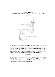
where G is the gravitational constant, M i is the mass, I the number of point massesand l i is the distance from the mass located at the point Q i to the point ofevaluation, P, see Fig. 1. The distance from the origin to P and Q i is denoted r P , r Qi ,respectively and the first will always be larger than the other. The angle (sphericaldistance) between the vectors to P and Q i is denoted ψ.PQFig. 1.We now drop the subscript on Q. The distance l, from P to Q is then l =r 2 P + r 2 Q − 2r P r Q cos (ψ). For the inverse distance we have∞1l = 1 r iQ Pr P r i (cosψ)Pi=0(2)where P i are the Legendre polynomials. Multipole-functions are derive from theinverse distance function by integration or differentiation (compare Tscherning andRapp (1974)), and will be denoted f.MT(P) = α i f i (P)i=1(3)MThe estimate T is determined so that ∑ i=1({L i T} − obs i ) 2 = min, where M is thenumber of observations and L i are the linear functionals associated with theobservations. In the computations described below we only consider heightanomalies (geoid heights), gravity disturbances and second-order radial derivatives.We intend to show that in order to make the functions suitable for regional gravityfield modeling low-degree terms may be removed or substituted by appropriateweights.

2. Higher order derivatives,For derivatives with respect to r P we have series expansions similar to eq. (2),where the terms for the first derivative are multiplied with –(i+1)/r P and for thesecond derivative with (i+1)*(i+2)/r P 2 . Closed expressions for the derivatives areeasily found.∂ 1 l= (r Qt − r P )∂r P l 3(4)∂ 2 1l∂r P2 = (3(r P − r Q t) 2 /l 2 − 1)/l 3(5)Point masses are not the only harmonic functions which may be used as basefunctions when approximating T, see e.g. Tscherning (1972), Hauck andLelgemann (1985) but we will only deal with point mass and excentric multipolesbase functions, since they fully represents the message of this paper.3. Reduced point masses.From eq. (2) we see that if we use the representation eq. (1), it will contain terms ofdegree zero and one, which are not present in T. So they have to be removed,simply by subtracting from the closed expressions the first two terms in eq. (2) orits derivative. (This is not done for the examples of closed expressions in section5). But what if we subtract from the data (and later add back) the contribution froma global model like EGM96, complete to degree N ?T N = GM r PNn=0 a nr Pncos(mλ) , m ≥ 0 C nm P nm (sinφ) sin(|m|λ) , m < 0 m=−n(6)Here φ is the geocentric latitude , λ the longitude, P nm the normalized Legendrefunctions and a a scale factor close to the semi-major axis. C nm are the normalized2Stokes coefficients with error-estimates σ nm . Degree-variances and error-degreevariancesare sums of the C nm squared, σ nm respectively, for a fixed degree, n,2multiplied with (GM/a) 2 .

As pointed out by Arabelos (1980) we can not simply put to zero the first N terms.Here a solution was found, i.e. that the first terms were not put to zero, but putequal to the so-called error-degree variances, σ 2 e,i contingently scaled by a factor αso as to reflect if the model was better (α≤1) or worse (α≥1) in an area.To get a little more insight into this, let us interpret the point mass potential as areproducing kernel in a Hilbert space, where the functions are harmonic down to aBjerhammar-sphere with radius R B inside the Earth and r Q < R B . Using a Kelvintransformation we obtain a point D outside the sphereR B2r P r D= r Qr P(7)So that L=1 − 2 R B 2cos(ψ) + R B 2 2 2Rr P r D r P r . Then K(P,D)= B/L is the so-calledD r P r DKrarup kernel, Krarup (1969). When interpreted as a covariance function, it hasunitless degree-variances equal to 1, i.e. it is not well suited to represent theanomalous potential, since the degree-variances of T tends to zero like n -3 * q, q

∞i=2A kF k r P , r Q, ψ = r i+1Q P(i − k) r i (cosψ)P(9)Each of these may be represented by a closed expression. The first termscorresponding to the maximal degree of the global model used, should besubstituted by the (scaled potential) error-degree-variances.Ncov N r P , r D, ψ = aσ iei=2 R B 2 i+1 Pr D r i (cosψ)P(10)5. Reduced point mass and excentric multipole base functions - examples.The interesting functions are those which represent the geoid (height anomaly) andthe first and second derivative with respect to r P . All quantities are anomalousquantities with respect to EGM96 complete to degree N=24. We consider geoidand gravity disturbance at height zero and the second order radial derivative at 250km altitude. For the latter we will put the mass-point at depth 242.5 km,corresponding to data (r P ) at 250 km. The Bjerhammar sphere will be put at 1.46km depth.In the first example (Table 1) we use as observation one (anomalous) radial gravitygradient observation equal to 0.15 Eötvöes, at height 250 km (M=1 in eq. (3)). Thelatitude and the longitude are set to zero for the mass-point, but the latitude for thepoint P increases in steps from zero. Table 2 shows the same function, now withthe quantities evaluated at zero altitude.In Table 3 we have corresponding values obtained using the covariance functioneq. (8), (10) and again with the same gravity gradient observation as used in Table1 and 2.We have here calculated values with spherical distance 1.0 degree and so that thevalue for the second order radial derivative is 0.15 Eötvös.

Table 1. Closed and Reduced Point mass functions at altitude 250 km. Note thelocation of the first zero-crossing. For the reduced function all terms up to degree24 have been set equal to zero.ψClosedexpressionReduced todeg. 24.Closed Reduced Closed ReducedGeoid (m)Gravitydisturbance(mgal)2. orderradial deriv.(Eötvös)0.0 0.85 0.29 -2.41 -1.79 0.150 0.1501.0 0.80 0.24 -2.03 -1.37 0.106 0.1002.0 0.70 0.14 -1.34 -0.62 0.043 0.0283.0 0.59 0.05 -0.81 -0.09 0.012 -0.0054.0 0.49 -0.02 -0.49 0.16 0.002 -0.0145.0 0.42 -0.05 -0.31 0.24 -0.001 0.0136.0 0.37 -0.05 -0.21 0.23 -0.002 -0.0107.0 0.32 -0.05 -0.14 0.17 -0.002 -0.0078.0 0.29 -0.03 -0.11 0.10 -0.001 -0.0039.0 0.26 -0.01 -0.10 0.01 -0.001 0.00010.0 0.23 0.00 -0.06 -0.02 0.000 0.002

Table 2. Closed and Reduced Point mass functions at zero altitude. Note thelocation of the first zero-crossing and the values for zero spherical distance. Thelocation is for the geoid at 3 0 . This corresponds (approximately) to the location ofthe first zero-point for the first Legendre polynomium in the series eq. (8).(Legendre polynomials have as many zero points as the degree in the interval from-90 0 to 90 0 distributed approximately equidistantly, see Heiskanen and Moritz,1967, Fig. 1-8).ψClosedexpressionReduced todeg. 24.Closed Reduced Closed ReducedGeoid (m)Gravitydisturbance(mgal)2. orderradialderiv.(Eötvös)0.0 3.56 3.13 -49.2 -55.3 13.9 16.11.0 1.93 1.24 -7.87 -7.26 -0.11 -0.182.0 1.09 0.31 -1.48 0.04 -0.14 -0.213.0 0.75 0.02 -0.51 0.98 -0.053 -0.10

Table 3. Values computed using a degree-variance model (eq.(8)) with depth to theBjerhammar-sphere equal to 1.56 km. Error.degree-variances from EGM96 used todegree 24, scaled with α= 1.03. Computed using Least-Squares-Collocation withonly one observation (completely equivalent to using eq. (3)).ψSecond order radialderivative. Altitude=250 km. Eöetvöesunits.Geoid. Zero altitude.Units m.Gravity anomaly.Zero altitude. Unitsmgal.0.0 0.15 2.11 13.111.0 0.13 1.80 10.362.0 0.08 1.23 5.333.0 0.03 0.46 1.404.0 -0.03 -0.04 -0.875.0 -0.03 -0.32 -1.866.0 -0.03 -0.43 -2.017.0 -0.02 -0.41 -1.668.0 -0.02 -0.30 -1.08Again we see the location of the first zero-crossing, which makes the function wellsuited for representing data where the contribution from EGM96 to degree 24 hasbeen subtracted.A FORTRAN program redpmass.f for doing these or similar calculations isavailable as http://cct.gfy.ku.dk/redpmass.f , 2010.05.20.4. Conclusion.Closed or reduced point mass or multipole functions may be used to represent theanomalous potential. When used regionally referring to a global gravity fieldmodel, the first terms must be removed or substituted by error-degree-variances.For point-mass or multipole functions the terms up to the lowest degree of thereference potential (the global model) have here been put equal to zero. However,it might be possible to find (unitless) terms representing the power in the

frequencies which the global model have not removed, corresponding to errordegreevariances.If covariance functions (corresponding to multipole base functions) are used, errordegree-variances (scaled) may be used. This assures that the model in anappropriate manner weights the regional frequencies with respect to the globalmodel used.References:Arabelos, D.: Untersuchungen zur gravimetrischen Geoidbestimmung, dargestelltam Testgebiet Griechenland. Wiss. Arb. d. Fachrichtung Vermessungswesen d.Universitaet Hannover, Hannover 1980.Ballani, L., J.Engel and E.Grafarend: Global base functions for the mass density inthe interior of a massive body (Earth), Manuscripta Geodaetica, Vol. 18, no. 2,pp. 99-114, 1993.Balmino, G.: La Representation du Potentielle par Masses Ponctuelles. BulletinGeodesique, No. 3, 1974.Barthelmes,F.: Untersuchungen zur Approximation des aeusserenGravitationsfeldes der Erde durch Punktmassen mit optimierten Positionen.Veroeff. Zentralinstituts fuer Physik der Erde, Nr. 92,Potsdam, DDR, 1986.Barthelmes,F. and H. Kautzleben: A New Method of Modelling the Gravity Fieldof the Earth by Point Masses. Proc. of the IAG Symposia, Vol.1, pp 442-448,Dep. of Geodetic Science and Surveying, The Ohio State University, 1983.Hauck, H. and D.Lelgemann: Regional gravity field approximation with buriedmasses using least-norm collocation. Manuscripta Geodaetica, Vol. 10, no. 1,pp. 50-58, 1985.Heiskanen, W.A. and H. Moritz: Physical Geodesy. W.H. Freeman & Co, SanFrancisco, 1967.Krarup, T.: A Contribution to the Mathematical Foundation of Physical Geodesy.Meddelelse no. 44, Geodætisk Institut, København 1969.Lemoine, F.G., S.C. Kenyon, J.K. Factor, R.G. Trimmer, N.K. Pavlis, D.S. Chinn,C.M. Cox, S.M. Klosko, S.B. Luthcke, M.H. Torrence, Y.M. Wang, R.G.Williamson, E.C. Pavlis, R.H. Rapp, and T.R. Olson, The Development of theJoint NASA GSFC and the National Imagery and Mapping Agency (NIMA)Geopotential Model EGM96, NASA/TP-1998-206861, Goddard Space FlightCenter, Greenbelt, MD, July, 1998.Marchenko, A.N., F.Barthelmes, U.Meyer and P.Schwintzer: Regional geoiddetermination: An application to airborne gravity data in the Skagerrak.STR01/07, GFZ Potsdam, 2001.