Elements of Statistical Methods Probability (Ch 3) - Statistics

Elements of Statistical MethodsProbability (Ch 3)Fritz ScholzSpring Quarter 2010April 5, 2010

Frequentist Interpretation of ProbabilityIn common language usage probability can take on several different meanings.E.g., there is the possibility, not necessarily certainty.There is a 40% chance that it will rain tomorrow.Given the current atmospheric conditions, under similar conditions in the pastit has rained the next day in about 40% of the cases.or: about 40% of the rain gauges in the forcast area showed rain.Both of these are examples of the frequentists’ notion of probability,in the long run what proportion of instances will give the target result?The 40% area forecast may need some thinking in that regard to make it fit.1

Subjectivist Interpretation of ProbabilityYou look out the window and say:there is a 40% chance that it rains while I walk to the train station.It is based on gut feeling (subjective) and internal vague memory of that person.Having received a high PSA value for a prostate checka man is 95% certain that the biopsy will show no cancer.A woman has to decide whether to undergo an operation.Based on medical experience (frequentist) it will be succesful in 40% of the cases.But she feels she has a better than 80% chance of success.It is my lucky day, I feel 70% certain that I will win something in the lottery.2

Observable EventsWe said that C should contain the observable events.What does observable mean?When S is finite we can take the collection C of all subsets of S.The same route can be taken with denumerable sample spaces S.When S = R, it is no longer so easy to take all possible subsets of R as C .We need to impose some axiomatic assumptions about C and P.5

Collection of Events: Required PropertiesAny collection C of events should satisfy the following properties:1. The sample space S is an event, i.e., S ∈ C2. If A is an event, i.e., A ∈ C , so is A c , i.e., A c ∈ C3. For any countable sequence of events, A 1 ,A 2 ,A 3 ... ∈ Ctheir union should also be an event, i.e., S ∞i=1A i ∈ C .Such a collection C with properties 1-3 is also called a sigma-fieldor sigma-algebra.By 1. and 2.: S ∈ C =⇒ S c = /0 ∈ C .C = {/0,S} is the simplest sigma-field.6

Coin Flips RevisitedSuppose we cannot distinguish HT and TH. Then we have as sample spaceS = {{H,H},{H,T},{T,T}}We used set notation to describe the three elements,order within a set is immaterial.As sigma-field of all subsets we get{C =S, /0, { {H,H} }, { {H,T} }, { {TT} },{ {H,H},{H,T} }, { {H,H},{T,T} }, { {T,T},{H,T} }}{ {H,H},{H,T} } c = { {TT} }The text treats this example within the context of the original sample space,but introduces the indistinguishability of HT and TH by imposing the conditionthat any event containing HT also contains TH.Compare the two models!7

The Probability Measure PA probability measure on C assigns a number P(A) to each event A ∈ Cand satisfies the following properties (axioms):1. For any A ∈ C we have 0 ≤ P(A) ≤ 1.2. P(S) = 1 The probability of some outcome in S happening is 1.3. For any sequence A 1 ,A 2 ,A 3 ,... of pairwise disjoint events we have( ) ( )[ ∞ ∞n[nP A i = ∑ P(A i ) i.e. P lim An→∞ i = limn→∞∑ P(A i )i=1 i=1i=1i=1The third property is referred to as countable additivity.8

P(/0) = 0This obvious property could have been added to the axioms, but it follows from 2-3.Consider the specific sequence of pairwise disjoint events S, /0, /0, /0,...and note that their infinite union is just S, i.e.,S ∪ /0 ∪ /0 ∪ /0 ∪ ··· = SFrom properties 2 and 3 (axioms 2 and 3) we have1 = P(S) = P(S ∪ /0 ∪ /0 ∪ /0 ∪ ···) = P(S) +∞∞∑ P(/0) = 1 + ∑ P(/0)i=2i=2it follows that ∑ ∞ i=2 P(/0) = 0 and thus P(/0) = 0. 9

Countable Additivity =⇒ Finite AdditivityLet A 1 ,...,A n be a finite sequence of pairwise disjoint events. ThenProof:P(A 1 ∪ ... ∪ A n ) = P( n [)A i =i=1n∑ P(A i ) = P(A 1 ) + ... + P(A n )i=1Augment the sequence A 1 ,...,A n with an infinite number of /0’s, then theinfinite sequence A 1 ,...,A n , /0, /0,... is pairwise disjoint and their union isA 1 ∪ ... ∪ A n ∪ /0 ∪ /0 ∪ ... =From axiom 3 together with P(/0) = 0 we getn[A ii=1P(A 1 ∪ ... ∪ A n ∪ /0 ∪ /0 ∪ ...) = P(A 1 ) + ... + P(A n ) + P(/0) + P(/0) + ...P(A 1 ∪ ... ∪ A n ) = P(A 1 ) + ... + P(A n )10

P(A c ) = 1 − P(A) & A ⊂ B =⇒ P(A) ≤ P(B)In both proofs below we use the established finite additivity property.S = A ∪ A c1 = P(S) = P(A) + P(A c ) =⇒ P(A c ) = 1 − P(A)Assume A ⊂ B, then A and B ∩ A c are mutually exclusive and their union is BB = A ∪ (B ∩ A c ) =⇒ P(B) = P(A) + P(B ∩ A c ) ≥ P(A)since P(B ∩ A c ) ≥ 0 by axiom 1.11

P(A ∪ B) = P(A) + P(B) − P(A ∩ B)For any A,B ∈ C we have the pairwise disjoint decompositions (see Venn diagram)A ∪ B = (A ∩ B c ) ∪ (A ∩ B) ∪ (B ∩ A c )=⇒ P(A ∪ B) = P(A ∩ B c ) + P(A ∩ B) + P(B ∩ A c )andA = (A ∩ B c ) ∪ (A ∩ B) and B = (A ∩ B) ∪ (B ∩ A c )=⇒ P(A) = P(A ∩ B c ) + P(A ∩ B) and P(B) = P(A ∩ B) + P(B ∩ A c )=⇒ P(A) + P(B) = P(A ∩ B c ) + 2P(A ∩ B) + P(B ∩ A c )= P(A ∪ B) + P(A ∩ B)=⇒ P(A) + P(B) − P(A ∩ B) = P(A ∪ B)12

Finite Sample SpacesSuppose S = {s 1 ,...,s N } is a finite sample space with outcomes s 1 ,...,s N .Assume that C is the collection of all subsets (events) of S.and that we have a probability measure P defined for all A ∈ C .Denote by p i = P({s i }) the probability of the event {s i }.Then for any event A consisting of outcomes s i1 ,...,s ik we have⎛ ⎞ ⎛ ⎞[P(A) = P⎝ k {s i j} ⎠ = P⎝ [{s i } ⎠ = ∑ P({s i }) = ∑ p i (1)s i ∈As i ∈Aj=1s i ∈AThe probabilities of the individual outcomes determine the probability of any event.To specify P on C , we only need to specify p 1 ,..., p N with 0 ≤ p i ,i = 1,...,Nand p 1 + ... + p N = 1.This together with (1) defines a probability measure on C , satisfying axioms 1-3.This also works for denumerable S with 0 ≤ p i ,i = 1,2,... and ∑ ∞ i=1 p i = 1.13

Equally Likely OutcomesMany useful probability models concern N equally likely outcomes, i.e.,p i = 1 N , i = 1,...,N Note p i ≥ 0 andFor such models the above event probability (1) becomesP(A) = ∑ p i = ∑s i ∈A s i ∈A1N = #(A)#(S)N∑ p i = Ni=1N = 1=# of cases favorable to A# of possible casesThus the calculation of probabilities is simply a matter of counting.14

Dice ExampleFor a pair of symmetric dice it seems reasonable to assume that all 36 outcomesin a proper roll of a pair of dice are equally likely.⎧(1,1) (1,2) (1,3) (1,4) (1,5) (1,6)⎪⎨. . . . . .S =. . . . . .⎪⎩(6,1) (6,2) (6,3) (6,4) (6,5) (6,6)⎫⎪⎬⎪⎭What is the chance of coming up with a 7 or 11?A = {(1,6),(2,5),(3,4),(4,3),(5,2),(6,1),(6,5),(5,6)}with #(A) = 8 and thus P(A) = 8/36 = 2/9.Counting by full enumeration can become tedious and shortcuts are desirable.15

Combinatorial Counts40 patients in a preliminary drug trial are equally split between men and women.We randomly split these 40 patients so that half get the new drugwhile the other half get a look alike placebo.What is the chance that the “new drug” patients are equally split between genders?“randomly split” means: any group of 20 out of 40 is equally likely to be selected.P(A) =( 2010) (×20)10) = choose(20,10)ˆ2/choose(40,20)( 4020= dhyper(10,20,20,20) = 0.2476289See documentation in R on using choose and dhyper.( 40) (Enumerating 20 = 137,846,528,820 and 20 210)= 184,7562 cases is impractical.16

Rolling 5 Fair Dicea) What is the probability that all 5 top faces show the same number?P(A) = 6 6 5 = 1 6 4 = 11296b) What is the probability that the top faces show exactly 4 different numbers?The duplicated number can occur on any one of the possible ( 52)pairs of dice(order does not matter) & these two identical numbers can be any one of 6 values.For the remaining 3 numbers we could have 5 × 4 × 3 possibilities. ThusP(A) = #(A)#(S) = 6 · (52)· 5 · 4 · 36 5 = 2554 = 0.462963We repeatedly made use of the multiplication principle in counting the combinationsof the various choices with each other.17

Rolling 5 Fair Dice (continued)c) What is the chance that the top faces show exactly three 6s or exactly two 5s?Let A = event of seeing exactly three 6s and B = event of seeing exactly two 5s?( 53)· 52( 52)· 53( 53)P(A) =6 5 , P(B) =6 5 , P(A ∩ B) =6 5P(A ∪ B) = P(A) + P(B) − P(A ∩ B) ==( 53)· 5 2 + ( 52)· 5 3 − ( 53)6 5250 + 1250 − 106 5 = 14906 5 ≈ 0.1916Sometimes you have to organize your counting in manageable chunks.18

The Birthday ProblemAssuming a 365 day year and dealing with a group of k students,what is the probability of having at least one birthday match among them?The basic operating assumption is that all 365 k birthday k-tuples (d 1 ,...,d k )are equally likely to have appeared in this class of k.We will employ a useful trick. Sometimes it is easier to get your countingarms around A c and then employ P(A) = 1 − P(A c ).A c means that all k birthdays are different.P(A c ) =365 · 364···(365 − (k − 1))365 · 364···(366 − k)365 k & P(A) = 1 −365 kIt takes just 23 students to get P(A) > .5.19

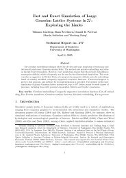
Matching or Adjacent BirthdaysWhat is the chance of having at least one matching or adjacent pair of birthdays?Again, going to the complement is easier. View Dec. 31 and Jan. 1 as adjacent.Let A be the event of getting n birthdays at least one day apart. Then we have( ) 365 − n − 1 (n − 1)!365P(A) =n − 1 365 n=(365 − 2n + 1)(365 − 2n + 2)···(365 − 2n + n − 1)365 n−1365 ways to pick a birthday for person 1. There are 365 − n non-birthdays (NB).Use the remaining n−1 birthdays ( (BD) to each fill one of the remaining 365−n−1365−n−1) gaps between the non-birthdays, n−1 ways.That fixes the circular NB–BD pattern, anchored on the BD of person 1.(n − 1)! ways to assigns these birthdays to the remaining (n − 1) persons.20

P(M) and P(A c )n = 14 gives the smallest n for which P(A c ) ≥ .5, in fact P(A c ) = .5375.probability0.0 0.2 0.4 0.6 0.8 1.0●●●●●●●●●●●●●●●●●●●●●●●●●●●●P(at least one matching B−day)P(at least one matching or adjacent B−day)●● ● ● ● ● ● ● ● ● ● ● ● ● ● ● ● ● ● ● ●●10 20 30 40 50number of persons n21

Conditional ProbabilityS● ● ●BA● ● ● ●● ● ●Conditional probabilities are a useful tool forbreaking down probability calculations intomanageable segments.The Venn diagram shows 10 equally likelyoutcomes and two events A and B.P(A) = #(A)#(S) = 3 10 = 0.3Suppose that we can restrict attention to theoutcomes in B as our new sample space, thenP(A|B) =#(A ∩ B)#(S ∩ B) = 1 5 = 0.2the conditional probability of A given B.22

Conditional Probability: Formal DefinitionThe previous example with equally likely outcomes can be rewritten asP(A|B) =#(A ∩ B)#(S ∩ B)=#(A ∩ B)/#(S)#(B)/#(S)which motivates the following definition in the general case,not restricted to equally likely outcomes=P(A ∩ B)P(B)Definition: When A and B are any events with P(B) > 0, then we define theconditional probability of A given B byP(A|B) =P(A ∩ B)P(B)This can be converted to the multiplication or product ruleP(A ∩ B) = P(A|B)P(B) and P(A ∩ B) = P(B ∩ A) = P(B|A)P(A)provided that in the latter case we have P(A) > 0.23

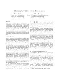
Two Headed/Tailed CoinsAsk Marilyn: Suppose that we have three coins, one with two heads on it (HH),one with two tails on it (TT) and a fair coin with head and tail (HT).One of the coins is selected at random and flipped. Suppose the face up is Heads.What is the chance that the other side is Heads as well?We could reason as follows:1. Given the provided information, it can’t be the TT coin. It must be HH or HT.2. If HH was selected face down is Heads, if HT then face down is Tails3. Thus the chance of having Heads as face down is 1/2. Or is it?24

Tree Diagramcoin=HH1up=H1down=H131312up=H1down=T161●3coin=HT1312up=T1down=H16coin=TT1up=T1down=T1325

Applying the Multiplication RuleP({up = H}) = P({{up = H} ∩ {coin = HH}} ∪ {{up = H} ∩ {coin = HT}})= P({up = H} ∩ {coin = HH}) + P({up = H} ∩ {coin = HT})= P({up = H}|{coin = HH}) · P({coin = HH})= 1 · 13 + 1 2 · 13 = 1 2+ P({up = H}|{coin = HT}) · P({coin = HT})P({down = H}|{up = H}) =P({up = H} ∩ {down = H})P({up = H})=P({coin = HH})1/2= 1/31/2 = 2 3 ≠ 1 226

HIV ScreeningA population can be divided into those that have HIV (denoted by D)and those who do not (denoted by D c ).A test either results in a positive, denoted by T + , or in a negative, denoted by T − .The Venn diagram shows the possible outcomes for a randomly chosen person.T +T −D D ∩ T + D ∩ T −D c D c ∩ T + D c ∩ T −Test is correct: D∩T + or D c ∩T − ; false positive: D c ∩T + ; false negative: D∩T − .27

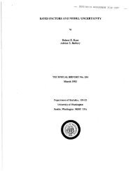
P(D|T + )?Typically something is known about the prevalence HIV, say P(D) = 0.001.We may also know P(T + |D c ) = 0.015 and P(T − |D) = .003,the respective probabilities of a false positive and a false negative.P(D|T + ) = P(D ∩ T + )P(T + )=P(D ∩ T + )P({T + ∩ D} ∪ {T + ∩ D c }) = P(D ∩ T + )P(T + ∩ D) + P(T + ∩ D c )==P(T + |D)P(D)P(T + |D)P(D) + P(T + |D c )P(D c )0.997 · 0.0010.997 · 0.001 + 0.015 · 0.999 = 0.06238 28

HIV Test Tree Diagram●0.0010.999T +0.997D0.003T −0.015T +D c0.001 × 0.9970.001 × 0.0030.999 × 0.0150.985T −0.999 × 0.985P(D | T + ) = P(D ∩ T+ )P(T + )=0.001 × 0.9970.001 × 0.997 + 0.999 × 0.015 = 0.06238268 29

IndependenceThe concept of independence is of great importance in probability and statistics.Informally: Two events are independent if the probability of occurrence of eitheris unaffected by the occurrence of the other.The most natural way is to express this via conditional probabilities as follows:orP(A|B) = P(A) and P(B|A) = P(B)P(A ∩ B)P(B)= P(A) andP(A ∩ B)P(A)Definition: Two events A and B are independent if and only ifP(A ∩ B) = P(A) · P(B)= P(B)Note that P(A) > 0 and P(B) > 0 are not required (as in P(B|A) and P(A|B)).30

Comments on IndependenceIf P(A) = 0 or P(B) = 0 then A and B are independent.Since A ∩ B ⊂ A and A ∩ B ⊂ B =⇒ 0 ≤ P(A ∩ B) ≤ min(P(A),P(B)) = 0, thus0 = P(A ∩ B) = P(A) · P(B) = 0If A∩B = /0, i.e., A and B are mutually exclusive, and P(A) > 0 and P(B) > 0, thenA and B cannot be independent.The fact that A and B are spatially uncoupled in the Venn diagram does not meanindependence, on the contrary there is strong dependence between A and BbecauseP(A ∩ B) = 0 < P(A) · P(B)or, knowing that A occurred, leaves no chance for B to occur (strong impact).Thus A and A c are not independent as long as 0 < P(A) < 1.31

Implied IndependenceIf A and B are independent so are A c and B and thus also A c and B c .Proof:P(B) = P(B ∩ A) + P(B ∩ A c ) = P(B) · P(A) + P(B ∩ A c )=⇒ P(B) · (1 − P(A)) = P(B ∩ A c ) =⇒ P(B ∩ A c ) = P(B)P(A c )32

Examples of Independence/Dependence1. Given: P(A) = 0.4, P(B) = 0.5, and P([A ∪ B] c ) = 0.3.Are A and B independent?P(A ∪ B) = 0.7 = P(A) + P(B) − P(A ∩ B) = 0.4 + 0.5 − P(A ∩ B)=⇒ P(A ∩ B) = 0.2 = P(A) · P(B) =⇒ A and B are independent!2. Given: P(A ∩ B c ) = 0.3, P(A c ∩ B) = 0.2, and P(A c ∩ B c ) = 0.1.Are A and B independent?0.1 = P(A c ∩ B c ) = P([A ∪ B] c ) = 1 − P(A ∪ B) =⇒ P(A ∪ B) = 0.90.9 = P(A ∪ B) = P(A ∩ B c ) + P(A c ∩ B) + P(A ∩ B) = 0.3 + 0.2 + P(A ∩ B)=⇒ P(A ∩ B) = 0.4 P(A) = 0.7 P(B) = 0.6and P(A ∩ B) = 0.4 ≠ P(A) · P(B) = 0.42, i.e., A and B are dependent.33

Postulated IndependenceIn practical applications independence is usually based on our understanding ofphysical independence, i.e., A relates to one aspect of an experiment while Brelates to another aspect that is physically independent from the former.In such cases we postulate probability models which reflect this independence.Example: First flip a penny, then spin it, with apparent physical independence.The sample space is S = {HH,HT,TH,TT}, with respective probabilitiesp 1 · p 2 , p 1 · (1 − p 2 ), (1 − p 1 ) · p 2 , (1 − p 1 ) · (1 − p 2 )where P(H on flip) = P({HT} ∪ {HH}) = p 1 · p 2 + p 1 · (1 − p 2 ) = p 1and P(H on spin) = P({TH} ∪ {HH}) = (1 − p 1 ) · p 2 + p 1 · p 2 = p 2and P({H on flip}∩{H on spin}) = P({HH}) = p 1 p 2 = P(H on flip)·P(H on spin)34

Common Dependence Situations1. Consider the population of undergraduates at William & Mary, from which astudent is selected at random. Let A be the event that the student is female,B be the event that the student is heading for elementary education.Being told P(A) ≈ .6 and P(A|B) ≥ .9 =⇒ A and B are not independent.2. Select a person at random from a population of registered voters.Let A be the event that the person belongs to a country club,B be the event that the person is a Republican. We probably would expectP(B|A) ≫ P(B)i.e., A and B are not independent.35

Mutual Independence of a Collection {A α } of EventsA collection {A α } of events is said to consist of mutually independent eventsif for any finite choice of events A α1 ,...,A αk in {A α } we haveP(A α1 ∩ ... ∩ A αk ) = P(A α1 ) · ... · P(A αk )For example, for 3 events A, B, C, we not only requireP(A ∩ B) = P(A) · P(B), P(A ∩C) = P(A) · P(C), P(B ∩C) = P(B) · P(C)but also P(A ∩ B ∩C) = P(A) · P(B) · P(C) (2)Pairwise independence does not necessarily imply (2).Counterexample: Flip 2 fair coins. Let A = {H on 1 st flip}, B = {H on 2 nd flip},C = {same result on both flips} with P(A) = P(B) = P(C) = 1 2andP(A ∩C) = P(HH) = 1 4 , etc., but P(A ∩ B ∩C) = P(HH) = 1 4 ≠ 1 8 .−→ text example on “independence” of 3 blood markers (O.J. Simpson trial).36

Random VariablesIn many experiments the focus is on numbers assigned to the various outcomes.Numbers → arithmetic and common arena for understanding experimental results.The simplest and nontrivial example is illustrated by a coin toss: S = {H,T},where we assign the number 1 to the outcome {H} and 0 to {T}.Such an assignment can be viewed as a function X : S → RHTX−→ 1 0with X(H) = 1 and X(T) = 0Such a function is called a random variable. We use capital letters from the end ofthe alphabet to denote such random variables (r.v.’s), e.g., U,V,W,X,Y,Z.Using the word “variable” to denote a function is somewhat unfortunate,but it is customary. It emphasizes the varying values that X can take onas a result of the (random) experiment.It seems that X only relabels the experimental outcomes, but there is more.37

Random Variables for Two Coin TossesToss a coin twice.Assign the number of heads to each outcome in S = {HH,HT,TH,TT}.Y : S → RHHTHHTTTY−→ 2 11 0with Y (HH) = 2, Y (HT) =Y (TH) = 1, and Y (TT) = 0We may also assign a pair of numbers (X 1 ,X 2 ) to each of the outcomes as followsX 1 (HH) = 1, X 1 (HT) = 1, X 1 (TH) = 0, X 1 (TT) = 0X 2 (HH) = 1, X 2 (HT) = 0, X 2 (TH) = 1, X 2 (TT) = 0X 1 = # of heads on the first toss and X 2 = # of heads on the second toss.X = (X 1 ,X 2 ) is called a random vector (of length 2).We can express Y also as Y = X 1 + X 2 = g(X 1 ,X 2 ) with g(x 1 ,x 2 ) = x 1 + x 2 .38

Borel SetsA random variable X induces a probability measure on a sigma field B of certainsubsets of R = (−∞,∞).This sigma field, the Borel sets, is the smallest sigma field containing all intervals(−∞,y] for y ∈ R, i.e., it contains all sets that can be obtained by complementation,countable unions and intersections of such intervals, e.g., it contains intervals like[a,b], [a,b), (a,b], (a,b) for any a,b ∈ R (why?)It takes a lot gyrations to construct a set that is not a Borel set.We won’t see any in this course.How do we assign probabilities to such Borel sets B ∈ B?Each r.v. X induces its own probability measure on the Borel sets B ∈ B.39

Induced Events and ProbabilitiesSuppose we have a r.v. X : S −→ R with corresponding probability space (S,C,P).For any Borel set B ∈ B we can determine the set X −1 (B) of all outcomes in Swhich get mapped into B, i.e.,X −1 (B) = {s ∈ S : X(s) ∈ B}How do we know that X −1 (B) ∈ C is an event?We don’t.Thus we require it in our definition of a random variable.Definition: A function X : S −→ R is a random variable if and only if theinduced event X −1 ((−∞,y]) ∈ C for any y ∈ Rand thus the induced probability P X (induced by P and X)P X ((−∞,y]) = P({s ∈ S : X(s) ≤ y})exists for all y ∈ R40

Cumulative Distribution Function (CDF)A variety of ways of expressing the same probability (relaxed and fastidious):()P X ((−∞,y]) = P X −1 ((−∞,y]) = P({s ∈ S : X(s) ∈ (−∞,y]})= P(−∞ < X ≤ y) = P(X ≤ y) (most relaxed)Definition: The cumulative distribution function (cdf) of a random variable Xis the function F : R −→ [0,1] defined byF(y) = P(X ≤ y)41

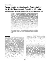
CDF for Single Coin Toss or Coin SpinExample (coin toss P(H) = 0.5):Since X takes only the values 1 and 0 for H and T we have⎧⎨ 0.0 = P(/0) for y < 0P(X ≤ y) = 0.5 = P(X = 0) = P(T) for 0 ≤ y < 1⎩1.0 = P(X = 0 ∪ X = 1) = P(T ∪ H) for 1 ≤ yExample (coin spin P(H) = 0.3):⎧⎨ 0.0 = P(/0) for y < 0P(X ≤ y) = 0.7 = P(X = 0) = P(T) for 0 ≤ y < 1⎩1.0 = P(X = 0 ∪ X = 1) = P(T ∪ H) for 1 ≤ yThe jump sizes at 0 and 1 represent 1 − P(H) = P(T) and P(H), respectively.See CDF plots on next slide.42

CDF for Coin Toss/Coin SpinF(y) = P(X ≤ y)0.0 0.2 0.4 0.6 0.8 1.0●●●●−2 −1 0 1 2 3yF(y) = P(X ≤ y)0.0 0.2 0.4 0.6 0.8 1.0●●●●−2 −1 0 1 2 343y

2 Fair Coin TossesFor two fair coin tosses the number X of heads takes the values 0,1,2for s = TT, s = HT or s = TH, and s = HH with probabilities 1 4 , 1 2 , 1 4 , respectively.P(X ≤ y) =⎧⎪⎨⎪⎩0.0 = P(/0) for y < 00.25 = P(X = 0) = P(TT) for 0 ≤ y < 10.75 = P(X = 0 ∪ X = 1) = P(TT ∪ HT ∪ TH) for 1 ≤ y < 21.0 = P(X = 0 ∪ X = 1 ∪ X = 2) = P(S) for 2 ≤ ySee CDF plot on next slide.44

CDF for 2 Fair Coin TossesF(y) = P(X ≤ y)0.0 0.2 0.4 0.6 0.8 1.0●●●●●●−2 −1 0 1 2 3y45

General CDF Properties1. 0 ≤ F(y) ≤ 1 for all y ∈ R (F(y) is a probability)2. y 1 ≤ y 2 =⇒ F(y 1 ) ≤ F(y 2 ) (monotonicity property)This follows since {X ≤ y 1 } ⊂ {X ≤ y 2 } =⇒ P(X ≤ y 1 ) ≤ P(X ≤ y 2 ).3. Limiting behavior as we approach ±∞lim F(y) = 0 and limy→−∞ y→∞ F(y) = 1This follows (with some more attention to technical detail) since\[lim {X ≤ y} = {X ≤ y} = /0 and lim {X ≤ y} = {X ≤ y} = Sy→−∞ y→∞y→−∞y→∞Note that in our examples we had F(y) = 0 for sufficiently low y (y < 0) andF(y) = 1 for sufficiently high y. X had a finite and thus bounded value set.46

Two Independent Random VariablesTwo random variable X 1 and X 2 are independent if any events defined in terms ofX 1 is independent of any event defined in terms of X 2 .The following weaker but more practical definition is equivalent.Definition: Let X 1 : S −→ R and X 2 : S −→ R be random variables defined on thesame sample space S. X 1 and X 2 are independent if and only if for each y 1 ∈ Rand y 2 ∈ RP(X 1 ≤ y 1 , X 2 ≤ y 2 ) = P(X 1 ≤ y 1 ) · P(X 2 ≤ y 2 )Note the shorthand notationP(X 1 ≤ y 1 , X 2 ≤ y 2 ) = P({X 1 ≤ y 1 } ∩ {X 2 ≤ y 2 })You also often see P(AB) for P(A ∩ B).47

Independent Random VariablesA collection of random variable {X α } is mutually independent if the above productproperty holds for any finite subsets of these random variables, i.e., for any integerk ≥ 2 and finite index subset α 1 ,...,α k we have for all y 1 ,...,y k ∈ RP(X α1 ≤ y 1 ,...,X αk ≤ y k ) = P(X α1 ≤ y 1 ) · ... · P(X αk ≤ y k )Whether the independence assumption is appropriate in a given applicationis mainly a matter of judgment or common sense.With independence we have access to many powerful and useful theoremsin probability and statistics.48