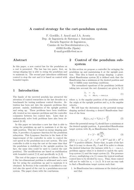
A control strategy for the cart-pendulum system Abstract 1 ...

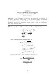
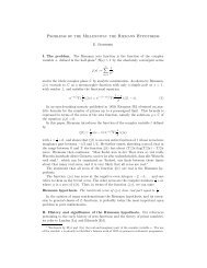
As ϕ is not definite, H d is not a Lyapunov functionin the whole state space. Consider now the followingLyapunov function candidate:V = ϕ(x 1 ,x 2 )(H d − 1/3)(= ϕ(x 1 ,x 2 ) − 1 3 cos3x 1 + 1 2 x2 2 − 1 ). (10)3Notice that V ≥ −2/3 and continuous. Nevertheless,V is not differentiable at the switching curve of (8).Outside this curve,This implies that:˙V = −ϕ 2 x 2 2 cos 2 x 1 ≤ 0• V is a Lyapunov function in the region Ω inside thecentral closed curve of Fig. 2. This closed curve isthe level curve V = 0.• The switching curve in (8) is attractive.In fact, a sliding motion is produced along the switchingcurve. The motion inside this curve can be deducedfrom the first equation of (9). Thus, only four equilibriain the sliding motion are possible (with x 1 ∈ [−π,π]):E 1,2 : (±π/3,0) and E 3,4 (±π,0). Besides, outside thesliding curve there are more limit sets: the maximuminvariant set in Ω for which ˙V = 0 is (±2π/3,0) ⋃ (0,0),being all equilibrium points. The latter is the desiredequilibrium while it is clear that the former ones areunstable. Therefore, the only problematic points areE 1,2 and E 3,4 .curves. It can be seen that the undesirable equilibriumpoints E 1,2 and E 3,4 still exist but they are outsidethe sliding manifold and, since they are unstable,they do not preclude the almost-global stability property.Nevertheless, this property is not proved yet. Noticethat with the choice (12), the Lyapunov functioncandidate is continuous along the dotted curve of Fig.3. But now, function ϕ ε introduces new switching linesat x 1 = ±π/3 (segments AB and CD in Fig. 3). Function(12) is not continuous at these segments and theanalysis must be performed carefully.In the following, it will be proved that, for smallenough ε, when the system reaches these points of discontinuityfor (12), the trajectory evolves towards theorigin. Due to the symmetry of the problem only thecase of x 2 > 0 will be considered. When the systemstarts on the upper half of segment AB as x 2 > 0 itwill evolve to the right. In this region Ḣd > 0 and thesystem will evolve towards the sliding curve (the dottedcurve of Fig. 3). After reaching x 1 = π it will continuefrom x 1 = −π towards x 1 = −π/3. Therefore, segmentCD (with x 2 > 0) will eventually be reached. When thesystem starts on this segment as x 2 > 0 it will evolvetowards the right but, in this region Ḣd < 0. If ε issmall enough the level curve H d = 1/3 (the solid curve)will be reached before reaching segment AB. Once thislevel curve is reached and crossed the system can not goout of the compact set {x : H d (x) < 1/3} where ˙V ≤ 0.1.512.2 Achieving almost-global stabilityIn order to avoid the undesirable equilibria E 1,2 andE 3,4 , the switching curve is changed from H d = 1/3 toH d = 1/3+ε with 0 < ε ≪ 1. This change is performedsubstituting the switching function ϕ byx 20.50−0.5−1CDAB{△ −k1 if Hϕ ε = d ≤ (1/3 + ε) and cosx 1 < 0.5k 1 elsewhereThe control law is now:u = 2sin 2x} {{ } 1 +ϕ ε (x 1 ,x 2 )x 2 cos x 1 (11)} {{ }u c u dThe same analysis can be performed with the Lyapunovfunction candidateV = ϕ ε (x 1 ,x 2 )(H d − 1/3 − ε) (12)The behaviour of the system can now be explained withthe help of Fig. 3. In this figure the level curves correspondingto H d = 1/3 and H d = 1/3 + ε are plotted.The sliding motion is now along the second of these−1.5−1 −0.8 −0.6 −0.4 −0.2 0 0.2 0.4 0.6 0.8 1x 1/πFigure 3: Level curves H d = 1/3 (solid) and H d =1/3 + ε (dotted)Since no other points of discontinuity exist, the followingproposition can be stated:Proposition 1. The origin of system (1) with controllaw (11) is almost globally asymptotically stable.2.3 Avoiding the sliding modeIn many control applications sliding modes are not admissibledue to the chattering phenomenon. The controllaw proposed in the previous section presents slidingmotions due to the discontinuity along the level curve3

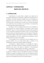
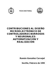
H d = 1/3 + ε. One way of solving this problem is proposedin this section. The idea is to modify the switchingfunction in such a way that it is equal to zero at bothsides of the switching curve. Thus, the switching functionwill be continuous at the switching curve and nosliding motions can occur. This can be accomplishedmultiplying function ϕ ε by abs(H d (x 1 ,x 2 ) − 1/3 − ε).In this way u d will be equal to zero at the level curveH d = 1/3+ε avoiding the sliding motion. Thus, the systemwill tend asymptotically to the former level curve.Since at x ∈ [−π/2,π/2] it is desired that the trajectoriescross the level curve, function ϕ ε should not changeat this interval. To this end we define a new switchingfunction:{△ k1 (H˜ϕ ε = d − 1/3 − ε) if cos x 1 < 0.5k 1elsewhere(13)The same previous analysis could be performed to thesystem with the control law derived from ˜ϕ ε . In orderto compute ˙V now, it must be taken into account that˜ϕ ε depends on x 1 and x 2 . It is easily seen that ˙V =−2˜ϕ 2 εx 2 2 cos 2 x 1 when cos x 1 < 0.5. Therefore V is stilla Lyapunov function.The behavioral difference with respect to the previouslaw is that the control law does not present antsliding motion. The cost of this nice nature is that theenergy injection/damping near the switching curve isvery small and, thus, the system will be slower. Theresultant control law is:u = 2sin 2x} {{ } 1 + ˜ϕ ε (x 1 ,x 2 )x 2 cos x 1 (14)} {{ }u c u dThe former discussion can be summarized in the followingresultProposition 2. Consider system (1) with control law(14) with ˜ϕ ε given by (13). Then, there exists a valueε ∗ > 0 such that if 0 < ε < ε ∗ the origin of the systemis almost globally asymptotically stable.2.4 SimulationsIn order to show the performance of control laws (11)and (14) Fig. 4 shows the simulation results of the systemwith both laws. Parameter k 1 is chosen to be equalto 3.0 and the initial conditions are set inside one ofthe undesirable wells. It can be seen that both controllaws are successful but that (11) is faster at the cost ofpresenting a sliding motion.2.5 Control of the cartIn the previous section only the movement of the pendulumwas considered whereas no control action wasdetermined in order to control the speed and the positionof the cart. In this section the previous controlx 2x 1ux 210−18642−1 −0.8 −0.6 −0.4 −0.2 0 0.2 0.4 0.6 0.8 1x 1/π00 2 4 6 8 10 12 14 16 18 20Time [s]50−50 2 4 6 8 10 12 14 16 18 20Time [s]x 1u10−14321a)−1 −0.8 −0.6 −0.4 −0.2 0 0.2 0.4 0.6 0.8 1x 1/π00 2 4 6 8 10 12 14 16 18 20Time [s]20−2−40 2 4 6 8 10 12 14 16 18 20Time [s]b)Figure 4: Results of a simulation with a) the slidingmode law and b) the modified law.law is modified (adding a new term) in such a way thatthe cart eventually stops while the pendulum is in theupright position.The model of the system when the cart speed dynamicsare considered [1] and after partial linearization [5]results:ẋ 1 = x 2ẋ 2 = sin x 1 − cos x 1 u (15)ẋ 3 = uwhere x 1 and x 2 have the same meaning as before, x 3is the cart speed.Notice that (15) is a feedforward system and, thus,forwarding can be applied. In order to avoid the resolutionof the partial differential equation, we will be basedon the partial state feeback stabilization with boundedcontrol variant [2,3].This method is intuitively suitable for the problemconsidered: the new control law will consist in a slightmodification of the control law that stabilizes the pen-4

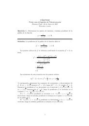
dulum and it will be expected that the deceleration ofthe pendulum will be slow. This is a very natural wayto work.In order to apply the method, consider system (15)with a control law that is the sum of previous modificationof control law (14) plus the new action u s (thesubscript stands for speed, since the aim of this term isto control the cart speed):ẋ 3 = 2sin 2x 1 + ˜ϕ ε x 2 cos x 1 + u s (16)ẋ 1 = x 2 (17)ẋ 2 = −sin 3x 1 − ˜ϕ ε x 2 cos 2 x 1 − cos x 1 u s , (18)which has been reordered as it is usual in the forwardingprocedure.Notice that in order to apply the method proposed in[2] subsystem (17)–(18) should be input-to-state stable(ISS). The basic idea is that, if this subsystem is ISS,then (x 1 ,x 2 ) will be sufficiently close to zero providedu s is small enough. Once this goal is accomplished allthe nonlinearities of the system can be approximatedby linear terms since all of them only depend on x 1and x 2 . The following proposition states the ISS (withrestrictions) property for this subsystem.Proposition 3. The system (17)–(18) is locally ISS for||x|| < 0.095π.Sketch of the proof The proof is only sketched here forthe lack of space. The idea is to choose as the Lyapunovfunction candidate the functionV (x 1 ,x 2 ) = − cos3 x 13+ 1 + 1 2 x2 2 + ε v2 x2 1 + ε v x 1 x 2 ,It can be seen that it fulfills the conditions of Theorem5.2 in [4] for ||x|| < 0.095π. ✷As we are interested in a global law that is even ableto swing up the pendulum, we have to include anotherdiscontinuity: we choose u s = 0 in order to reach theregion for which system (17)–(18) is locally ISS. Oncethis region is reached, we choose u S as below in order toalso stabilize (16) according to the procedure proposedin [2].Due to the ISS property and to the fact that u s issmall, variables x 1 and x 2 will eventually approach tozero and, then, we can use a linear approximation for allthe nonlinear functions that appear in the model sincex 3 does not appear in them. The method proposes thefollowing control law:( )l3 x 3u s = ε k σ(19)ε kwhere σ denotes the normalized saturation σ(·) =sign(·)min{| · |,1} and l 3 is a parameter that can betuned considering only the linear approximation of theresultant system. Notice that this control law fulfills ourrequirement: is bounded by ε k . The fact that, with u k ,x 3 tends to zero when x 1 and x 2 are close to zero can bededuced from the circle criterion: using the linear approximationof the nonlinearities that depend only onx 1 and x 2 , the only remaining nonlinearity is the oneintroduced in (19). It can be seen that the system is inLur’e form and, thus, the circle criterion can be applied.The system is:with⎡A = ⎣ẋ = Ax + Buy = Cx (20)( )l3 x 3u = ε k σε k0 1 0−3 −k 1 04 k 1 0⎤⎡⎦ B = ⎣0−11and C = [0 0 1]. Since u k belongs to the sector (0,l 3 ],system (20) will be asymptotically stable if G(jω) =−C(jωI − A) −1 B (the minus sign is due to the usualnegative feedback) lies on the right of the vertical linegoing through (−1/l 3 ,0). It can be seen that the locusG(jω) is bounded from the left and, thus, for smallenough values of l 3 the stability is guaranteed.In summary, the resultant control law is given by:u = u e + u swhere u e = u c + u d is given in (14) and u s is given by{0( ) for ||x|| ≥ 0.095πu s = lε k σ 3x 3(21)ε kfor ||x|| < 0.095πSince u e introduces a discontinuity, the final controlsignal will have two points of discontinuity: the first onewhen x 1 crosses one of the values ± π 3and the secondone when (x 1 ,x 2 ) enters the central region of Fig. 2. Ifε is small enough and following the reasoning of Section2.2 these each of these two situations can occur only onetime in one orbit. Notice that the gap of both discontinuitiescan be made arbitrarily small reducing ε and ε k .However, making ε k small deteriorates the performanceof the system.It should be realized that the ideas of [3,7,8] can berecursively applied and, thus, the position of the cartcould also be controlled in a further step. Nevertheless,for simplicity, this step is omitted here.The performance of the proposed strategy can be observedin the simulation that appears in Fig. 5 whichcorresponds to the values x(0) = (0.99π,0,0), ε = 0.1,k 1 = 5, ε k = 0.2, ε v = 0.1, l 3 = 1. The top left graphshows the projection of the trajectory into the (x 1 ,x 2 )plane. It can be seen that, in a first stage, the trajectoryreaches a neighborhood of the origin of this plane.⎤⎦ ,5

The final behavior is better seen in the top right graphwhere the time evolutions of x 1 and x 3 are plotted (x 2is omitted for clarity). It can be seen that the threevariables (and, consequently, also x 2 ) eventually tendto zero. The bottom left graph shows the evolution ofu, which is zoomed in the bottom right graph, showingthe two discontinuities.x 20.50−0.5−1−1.5−0.5 0 0.5 1x /π 1u210−1−2−30 5 10 15 20Time3 Conclusionsu43210−1−2−30 5 10 15 20Time1.510.50−0.5−1−1.5Figure 5: Simulation results.x 1x 3−20 2 4 6 8TimeIn this paper we have presented a new control strategyfor the well-known pendulum-on-a-cart system. Thenovelty of the new strategy is, on the one hand, the factthat it is able to swing up and to maintain the pendulum;on the other hand the cart speed is also controlled.Furthermore, the same procedure can be extended toalso control the position of the cart.Most of the laws presented in the literature control thecart only once the pendulum has been swang up by commutingto another control law. The law presented herepresents, at most, two discontinuities for each orbit butit has the nice characteristic of not commuting betweendifferent control laws based on different approaches.[2] G. Kaliora and A. Astolfi. A simple design for thestabilization of a class of cascaded nonlinear systemswith bounded control. In Proceedings of the40th IEEE Conference on Decision and Control,pages 3784–3789, 2001.[3] Georgia Kaliora. Control of nonlinear systems withbounded signals. PhD thesis, Imperial College ofSicnece, Technology and Medicine, London, 2002.[4] H. K. Khalil. Nonlinear Systems. Prentice Hall,second edition, 1996.[5] M. W. Spong. Energy based control of a class ofunderatuated mechanical systems. In Proceedingsof the 13th World Congress of the IFAC, pages 431–435, 1996.[6] B. Srinivasan, P. Huguenin, K. Guemghar, andD. Bonvin. A global stabilization strategy for an invertedpendulum. In Proceedings of the 15th WorldCongress of the IFAC, 2002.[7] A. R. Teel. Feedback stabilization: Nonlinear solutionsto inherently nonlinear problems. PhD thesis,University of California at Berkeley, 1992.[8] A. R. Teel. Global stabilization and restrictedtracking for multiple integrators with bounded control.Systems and Control Letters, 18(3):165–171,1992.[9] A. van der Schaft. L 2 -Gain and Passivity Techniquesin Nonlinear Control. Springer-Verlag, 1989.[10] J. Zhao and M. W. Spong. Hybrid control for globalstabilization of the cart-pendulum system. Automatica,37:1941–1951, 2001.AcknowledgmentsThis work has been supported under MCyT-FEDERgrants DPI2003-00429 and DPI2001-2424-C02-01.References[1] I. Fantoni and R. Lozano. Non-linear control forunderactuated mechanical systems. Springer, London,2002.6