What Is Optimization Toolbox?

Optimization Toolbox 3User’s Guide

How to Contact The MathWorkswww.mathworks.comWebcomp.soft-sys.matlabNewsgroupwww.mathworks.com/contact_TS.html Technical Supportsuggest@mathworks.combugs@mathworks.comdoc@mathworks.comservice@mathworks.cominfo@mathworks.com508-647-7000 (Phone)508-647-7001 (Fax)The MathWorks, Inc.3 Apple Hill DriveNatick, MA 01760-2098Product enhancement suggestionsBug reportsDocumentation error reportsOrder status, license renewals, passcodesSales, pricing, and general informationFor contact information about worldwide offices, see the MathWorks Web site.Optimization Toolbox User’s Guide© COPYRIGHT 1990–2007 by The MathWorks, Inc.The software described in this document is furnished under a license agreement. The software may be usedor copied only under the terms of the license agreement. No part of this manual may be photocopied orreproduced in any form without prior written consent from The MathWorks, Inc.FEDERAL ACQUISITION: This provision applies to all acquisitions of the Program and Documentationby, for, or through the federal government of the United States. By accepting delivery of the Program orDocumentation, the government hereby agrees that this software or documentation qualifies as commercialcomputer software or commercial computer software documentation as such terms are used or definedin FAR 12.212, DFARS Part 227.72, and DFARS 252.227-7014. Accordingly, the terms and conditions ofthis Agreement and only those rights specified in this Agreement, shall pertain to and govern the use,modification, reproduction, release, performance, display, and disclosure of the Program and Documentationby the federal government (or other entity acquiring for or through the federal government) and shallsupersede any conflicting contractual terms or conditions. If this License fails to meet the government’sneeds or is inconsistent in any respect with federal procurement law, the government agrees to return theProgram and Documentation, unused, to The MathWorks, Inc.TrademarksMATLAB, Simulink, Stateflow, Handle Graphics, Real-Time Workshop, and xPC TargetBoxare registered trademarks, and SimBiology, SimEvents, and SimHydraulics are trademarks ofThe MathWorks, Inc.Other product or brand names are trademarks or registered trademarks of their respectiveholders.PatentsThe MathWorks products are protected by one or more U.S. patents. Please seewww.mathworks.com/patents for more information.

Revision HistoryNovember 1990 First printingDecember 1996 Second printing For MATLAB 5January 1999 Third printing For Version 2 (Release 11)September 2000 Fourth printing For Version 2.1 (Release 12)June 2001 Online only Revised for Version 2.1.1 (Release 12.1)September 2003 Online only Revised for Version 2.3 (Release 13SP1)June 2004 Fifth printing Revised for Version 3.0 (Release 14)October 2004 Online only Revised for Version 3.0.1 (Release 14SP1)March 2005 Online only Revised for Version 3.0.2 (Release 14SP2)September 2005 Online only Revised for Version 3.0.3 (Release 14SP3)March 2006 Online only Revised for Version 3.0.4 (Release 2006a)September 2006 Sixth printing Revised for Version 3.1 (Release 2006b)March 2007 Seventh printing Revised for Version 3.1.1 (Release 2007a)

AcknowledgmentsAcknowledgmentsTheMathWorkswouldliketoacknowledgethefollowingcontributorstoOptimization Toolbox.Thomas F. Coleman researched and contributed the large-scale algorithmsfor constrained and unconstrained minimization, nonlinear least squares andcurve fitting, constrained linear least squares, quadratic programming, andnonlinear equations.Dr. Coleman is Dean of Faculty of Mathematics and Professor ofCombinatorics and Optimization at University of Waterloo.Dr. Coleman has published 4 books and over 70 technical papers in theareas of continuous optimization and computational methods and tools forlarge-scale problems.Yin Zhang researched and contributed the large-scale linear programmingalgorithm.Dr. Zhang is Professor of Computational and Applied Mathematics on thefaculty of the Keck Center for Interdisciplinary Bioscience Training at RiceUniversity.Dr. Zhang has published over 50 technical papers in the areas of interior-pointmethods for linear programming and computation mathematicalprogramming.

Acknowledgments

Contents1Getting StartedWhat Is Optimization Toolbox? ...................... 1-2Introduction ...................................... 1-2Optimization Functions ............................ 1-2Optimization Toolbox GUI .......................... 1-2Optimization Example ............................. 1-4The Problem ..................................... 1-4Setting Up the Problem ............................ 1-4Finding the Solution ............................... 1-5More Examples ................................... 1-62TutorialIntroduction ...................................... 2-3Problems Covered by the Toolbox ..................... 2-3Using the Optimization Functions .................... 2-6Medium- and Large-Scale Algorithms ................. 2-7Examples That Use Standard Algorithms ............ 2-9Introduction ...................................... 2-9Unconstrained Minimization Example ................ 2-10Nonlinear Inequality Constrained Example ............ 2-12Constrained Example with Bounds ................... 2-13Constrained Example with Gradients ................. 2-15Gradient Check: Analytic Versus Numeric ............. 2-17Equality Constrained Example ...................... 2-18Maximization ..................................... 2-19Greater-Than-Zero Constraints ...................... 2-19Avoiding Global Variables via Anonymous and NestedFunctions ...................................... 2-20Nonlinear Equations with Analytic Jacobian ........... 2-22vii

Nonlinear Equations with Finite-Difference Jacobian .... 2-25Multiobjective Examples ............................ 2-26Large-Scale Examples .............................. 2-40Introduction ...................................... 2-40Problems Covered by Large-Scale Methods ............. 2-41Nonlinear Equations with Jacobian ................... 2-45Nonlinear Equations with Jacobian Sparsity Pattern .... 2-47Nonlinear Least-Squares with Full Jacobian SparsityPattern ........................................ 2-50Nonlinear Minimization with Gradient and Hessian ..... 2-51Nonlinear Minimization with Gradient and HessianSparsity Pattern ................................ 2-53Nonlinear Minimization with Bound Constraints andBanded Preconditioner ........................... 2-55Nonlinear Minimization with Equality Constraints ...... 2-59Nonlinear Minimization with a Dense but StructuredHessian and Equality Constraints .................. 2-61Quadratic Minimization with Bound Constraints ....... 2-65Quadratic Minimization with a Dense but StructuredHessian ....................................... 2-67Linear Least-Squares with Bound Constraints .......... 2-72Linear Programming with Equalities and Inequalities ... 2-73Linear Programming with Dense Columns in theEqualities ..................................... 2-75Default Options Settings ........................... 2-78Introduction ...................................... 2-78Changing the Default Settings ....................... 2-78Displaying Iterative Output ........................ 2-81Most Common Output Headings ..................... 2-81Function-Specific Output Headings ................... 2-82Calling an Output Function Iteratively .............. 2-88What the Example Does ............................ 2-88Output Function .................................. 2-89Creating the M-File for the Example .................. 2-90Running the Example .............................. 2-92Optimizing Anonymous Functions Instead ofM-Files ......................................... 2-95viiiContents

Other Examples That Use this Technique .............. 2-96Typical Problems and How to Deal with Them ....... 2-98Selected Bibliography .............................. 2-1023Standard AlgorithmsOptimization Overview ............................ 3-4Demos of Medium-Scale Methods ................... 3-5Unconstrained Optimization ........................ 3-6Introduction ...................................... 3-6Quasi-Newton Methods ............................ 3-7Line Search ...................................... 3-9Quasi-Newton Implementation ...................... 3-11Hessian Update ................................... 3-11Line Search Procedures ............................ 3-11Least-Squares Optimization ........................ 3-18Introduction ...................................... 3-18Gauss-Newton Method ............................. 3-20Levenberg-Marquardt Method ....................... 3-21Nonlinear Least-Squares Implementation ............. 3-22Nonlinear Systems of Equations .................... 3-25Introduction ...................................... 3-25Gauss-Newton Method ............................. 3-25Trust-Region Dogleg Method ........................ 3-25Nonlinear Equations Implementation ................. 3-27Constrained Optimization .......................... 3-29Introduction ...................................... 3-29Sequential Quadratic Programming (SQP) ............. 3-30ix

Quadratic Programming (QP) Subproblem ............. 3-31SQP Implementation .............................. 3-32Simplex Algorithm ................................ 3-39Multiobjective Optimization ........................ 3-43Introduction ...................................... 3-43Weighted Sum Method ............................. 3-46Epsilon-Constraint Method ......................... 3-47Goal Attainment Method ........................... 3-49Algorithm Improvements for the Goal AttainmentMethod ........................................ 3-50Selected Bibliography .............................. 3-534Large-Scale AlgorithmsTrust-Region Methods for Nonlinear Minimization ... 4-3Demos of Large-Scale Methods ...................... 4-6Preconditioned Conjugate Gradients ................ 4-7Algorithm ........................................ 4-7Linearly ConstrainedProblems ..................... 4-9Linear Equality Constraints ......................... 4-9Box Constraints ................................... 4-10Nonlinear Least-Squares ........................... 4-12Quadratic Programming ........................... 4-13Linear Least-Squares .............................. 4-14Large-Scale Linear Programming ................... 4-15Introduction ...................................... 4-15xContents

Main Algorithm ................................... 4-15Preprocessing .................................... 4-18Selected Bibliography .............................. 4-205Optimization ToolGetting Started with the Optimization Tool .......... 5-2Introduction ...................................... 5-2Opening the Optimization Tool ...................... 5-2Steps for Using the Optimization Tool ................. 5-4Selecting a Solver ................................. 5-5Defining the Problem .............................. 5-7Introduction ...................................... 5-7bintprog Problem Setup ............................ 5-8fgoalattain Problem Setup .......................... 5-10fminbnd Problem Setup ............................ 5-11fmincon Problem Setup ............................. 5-12fminimax Problem Setup ........................... 5-14fminsearch Problem Setup .......................... 5-15fminunc Problem Setup ............................ 5-16fseminf Problem Setup ............................. 5-17fsolve Problem Setup ............................... 5-18fzero Problem Setup ............................... 5-19linprog ProblemSetup ............................. 5-20lsqcurvefit Problem Setup .......................... 5-22lsqlin Problem Setup ............................... 5-23lsqnonlin Problem Setup ............................ 5-24lsqnonneg Problem Setup ........................... 5-25quadprog Problem Setup ........................... 5-26Running a Problem in the Optimization Tool ......... 5-28Introduction ...................................... 5-28Pausing and Stopping the Algorithm .................. 5-28Viewing Results ................................... 5-29Final Point ....................................... 5-29xi

Specifying the Options ............................. 5-30Stopping Criteria .................................. 5-30Function Value Check .............................. 5-32User-Supplied Derivatives .......................... 5-32Approximated Derivatives .......................... 5-33Algorithm Settings ................................ 5-34Multiobjective Problem Settings ..................... 5-37Inner Iteration Stopping Criteria ..................... 5-37Plot Functions .................................... 5-39Output function ................................... 5-40Display to Command Window ....................... 5-40Getting Help in the Optimization Tool ............... 5-42Quick Reference ................................... 5-42Additional Help ................................... 5-42Importing and Exporting Your Work ................ 5-43Starting a New Problem ............................ 5-43Exporting to the MATLAB Workspace ................. 5-44Generating an M-File .............................. 5-45Closing the Optimization Tool ....................... 5-46Importing Your Work .............................. 5-46Optimization Tool Examples ........................ 5-47Optimization Tool with the fmincon Solver ............. 5-47Optimization Tool with the lsqlin Solver ............... 5-516Argument and Options ReferenceFunction Arguments ............................... 6-2Optimization Options .............................. 6-8Options Structure ................................. 6-8Output Function .................................. 6-16Plot Functions .................................... 6-25xiiContents

7Functions — By CategoryMinimization ...................................... 7-2Equation Solving .................................. 7-2Least Squares (Curve Fitting) ....................... 7-3Graphical User Interface ........................... 7-3Utility ............................................ 7-38Functions — Alphabetical ListIndexxiii

xivContents

1Getting StartedWhat Is Optimization Toolbox?(p. 1-2)Optimization Example (p. 1-4)Introduces the toolbox and describesthe types of problems it is designedto solve.Presents an example that illustrateshow to use the toolbox.

1 Getting StartedWhat Is Optimization Toolbox?• “Introduction” on page 1-2• “Optimization Functions” on page 1-2• “Optimization Toolbox GUI” on page 1-2IntroductionOptimization Toolbox extends the capability of the MATLAB ® numericcomputing environment. The toolbox includes routines for many types ofoptimization including• Unconstrained nonlinear minimization• Constrained nonlinear minimization, including goal attainment problems,minimax problems, and semi-infinite minimization problems• Quadratic and linear programming• Nonlinear least-squares and curve fitting• Nonlinear system of equation solving• Constrained linear least squares• Sparse and structured large-scale problemsOptimization FunctionsAll the toolbox functions are MATLAB M-files, made up of MATLABstatements that implement specialized optimization algorithms. You can viewthe MATLAB code for these functions using the statementtype function_nameYou can extend the capabilities of Optimization Toolbox by writing your ownM-files, or by using the toolbox in combination with other toolboxes, or withMATLAB or Simulink ® .Optimization Toolbox GUIThe Optimization Tool (optimtool) is a GUI for selecting a solver, specifyingthe optimization options, and running problems. You can define and modify1-2

What Is Optimization Toolbox?problems quickly with the GUI. You can also import and export from theMATLAB workspace and generate M-files containing your configuration forthe solver and options.1-3

1 Getting StartedOptimization ExampleThis section presents an example that illustrates how to solve an optimizationproblem using the toolbox function lsqlin, which solves linear least squaresproblems. This section covers the following topics:• “The Problem” on page 1-4• “Setting Up the Problem” on page 1-4• “Finding the Solution” on page 1-5• “More Examples” on page 1-6The ProblemThe problem in this example is to find the point on the planethat is closest to the origin. The easiest way to solve this problem is tominimize the square of the distance from a pointon the planeto the origin, which returns the same optimal point as minimizing the actualdistance. Since the square of the distance from an arbitrary pointto the origin is, you can describe the problem as follows:subject to the constraintThe function f(x) iscalledtheobjective function andis anequality constraint. More complicated problems might contain other equalityconstraints, inequality constraints, and upper or lower bound constraints.Setting Up the ProblemThis section shows how to set up the problem before applying the functionlsqlin, which solves linear least squares problems of the following form:1-4

Optimization Examplewhereis the norm of Cx - d squared, subject to the constraintsTo set up the problem, you must create variables for the parameters C, d, A,b, Aeq, andbeq. lsqlin accepts these variables as input arguments withthe following syntax:x = lsqlin(C, d, A, b, Aeq, beq)To create the variables, do the following steps:Create Variables for the Objective Function1 Since you want to minimize , you can set C to be the3-by-3 identity matrix and d tobea3-by-1vectorofzeros,sothatCx - d = x.C = eye(3);d = zeros(3,1);Create Variables for the Constraints2 Since this example has no inequality constraints, you can set A and b to beempty matrices in the input arguments.You can represent the equality constraintform asin matrixwhere Aeq =[124]andbeq = [7]. To create variables for Aeq and beq, enterAeq = [1 2 4];beq = [7];Finding the SolutionTo solve the optimization problem, enter1-5

1 Getting Started[x, fval] =lsqlin(C, d, [], [], Aeq, beq)lsqlin returnsx =0.33330.66671.3333fval =2.3333The minimum occurs at the point x and fval isthesquareofthedistancefrom x to the origin.Note In this example, lsqlin issues a warning that it is switching from itsdefault large-scale algorithm to its medium-scale algorithm. This message hasno bearing on the result, so you can safely ignore it. “Using the OptimizationFunctions” on page 2-6 provides more information on large- and medium-scalealgorithms.More ExamplesThe following sections contain more examples of solving optimizationproblems:• “Examples That Use Standard Algorithms” on page 2-9• “Large-Scale Examples” on page 2-40• Optimization Tool Example contains the example shown above for lsqlinusing the Optimization Tool.1-6

2TutorialThe Tutorial provides information on how to use the toolbox functions. It alsoprovides examples for solving different optimization problems.Introduction (p. 2-3)Examples That Use StandardAlgorithms (p. 2-9)Summarizes, in tabular form,functions available for minimization,equation solving, and solvingleast-squares or data fittingproblems. It also provides basicguidelines for using optimizationroutines and introduces algorithmsand line-search strategies availablefor solving medium- and large-scaleproblems.Presents medium-scale algorithmsthrough a selection of minimizationexamples. These examples includeunconstrained and constrainedproblems,aswellasproblemswith and without user-suppliedgradients. This section also discussesmaximization, greater-than-zeroconstraints, passing additionalarguments, and multiobjectiveexamples.

2 TutorialLarge-Scale Examples (p. 2-40)Default Options Settings (p. 2-78)Displaying Iterative Output (p. 2-81)Calling an Output FunctionIteratively (p. 2-88)Optimizing Anonymous FunctionsInstead of M-Files (p. 2-95)Typical Problems and How to Dealwith Them (p. 2-98)Selected Bibliography (p. 2-102)Presents large-scale algorithmsthrough a selection of large-scaleexamples. These examples includespecifying sparsity structures,and preconditioners, as well asunconstrained and constrainedproblems.Describes the use of default optionssettings, how to change them andhow to determine which options areused by a specified function. It alsoIncludes examples of setting somecommonly used options.Describes iterative output you candisplay in the Command Window.Describes how to make anoptimization function call anoutput function at each iteration.Describes how to represent amathematical function at thecommand line by creating ananonymous function from a stringexpression. It also includes anexample for passing additionalparameters.Provides tips to improve solutionsfound using optimization functions,improve efficiency of algorithms,overcome common difficulties, andtransform problems typically not instandard form.Lists published materials thatsupport concepts implemented inOptimization Toolbox.2-2

IntroductionIntroductionOptimization is the process of finding the minimum or maximum of a function,usually called the objective function. Optimization Toolbox consists offunctions that perform minimization (or maximization) on general nonlinearfunctions. The toolbox also provides functions for nonlinear equation solvingand least-squares (data-fitting) problems.This introduction includes the following sections:• “Problems Covered by the Toolbox” on page 2-3• “Using the Optimization Functions” on page 2-6• “Medium- and Large-Scale Algorithms” on page 2-7Problems Covered by the ToolboxThe following tables show the functions available for minimization, equationsolving, binary integer programming problems, and solving least-squares ordata-fitting problems.MinimizationType Notation FunctionScalar minimizationsuch thatfminbndUnconstrained minimizationfminunc,fminsearchLinear programmingsuch thatlinprogQuadratic programmingsuch thatquadprog2-3

2 TutorialMinimization (Continued)Type Notation FunctionConstrained minimizationsuch thatfminconGoal attainmentfgoalattainsuch thatMinimaxsuch thatfminimaxSemi-infinite minimizationsuch thatfseminfBinary integer programmingbintprog2-4

IntroductionEquation SolvingType Notation FunctionLinear equations, n equations, n \ (matrix left division)variablesNonlinear equation of onevariableNonlinear equations, n equations, nvariablesfzerofsolveLeast-Squares (Curve Fitting)Type Notation FunctionLinear least-squares\ (matrix left, m equations, n variables division)Nonnegativelinear-least-squaressuch thatlsqnonnegConstrainedlinear-least-squaressuch thatlsqlinNonlinear least-squaressuch thatlsqnonlinNonlinear curve fittingsuch thatlsqcurvefit2-5

2 TutorialUsing the Optimization FunctionsThis section provides some basic information about using the optimizationfunctions.Defining the Objective FunctionMany of the optimization functions require you to create a MATLAB functionthat computes the objective function. The function should accept vectorinputs and return a scalar output of type double. Therearetwowaystocreate the objective function:• Create an anonymous function at the command line. For example, to createan anonymous function for x 2 ,entersquare = @(x) x.^2;Youthencallthe optimization function with square as the first inputargument. You can use this method if the objective function is relativelysimple and you do not need to use it again in a future MATLAB session.• Write an M-file for the function. For example, to write the function x 2 as aM-file, open a new file in the MATLAB editor and enter the following code:function y = square(x)y = x.^2;You can then call the optimization function with @square as the first inputargument. The @ sign creates a function handle for square. Use thismethod if the objective function is complicated or you plan to use it formore than one MATLAB session.Note Because the functions in Optimization Toolbox only accept inputs oftype double, user-supplied objective and nonlinear constraint functions mustreturn outputs of type double.Maximizing Versus MinimizingThe optimization functions in the toolbox minimize the objective function. Tomaximize a function f, apply an optimization function to minimize -f. The2-6

Introductionresulting point where the maximum of f occurs is also the point where theminimum of -f occurs.Changing OptionsYou can change the default options for an optimization function by passingin an options structure, which you create using the function optimset, asan input argument. See “Default Options Settings” on page 2-78 for moreinformation.Supplying the GradientMany of the optimization functions use the gradient of the objective functionto search for the minimum. You can write a function that computes thegradient and pass it to an optimization function using the options structure.“Constrained Example with Gradients” onpage2-15providesanexampleofhow to do this. Providing a gradient function improves the accuracy and speedof the optimization function. However, for some objective functions it mightnot be possible to provide a gradient function, in which case the optimizationfunction calculates it using an adaptive finite-difference method.Medium- and Large-Scale AlgorithmsThis guide separates “medium-scale” algorithms from “large-scale”algorithms. Medium-scale is not a standard term and is used here only todistinguish these algorithms from the large-scale algorithms, which aredesigned to handle large-scale problems efficiently.Medium-Scale AlgorithmsOptimization Toolbox routines offer a choice of algorithms and line searchstrategies. The principal algorithms for unconstrained minimization arethe Nelder-Mead simplex search method and the BFGS (Broyden, Fletcher,Goldfarb, and Shanno) quasi-Newton method. For constrained minimization,minimax, goal attainment, and semi-infinite optimization, variations ofsequential quadratic programming (SQP) are used. Nonlinear least-squaresproblems use the Gauss-Newton and Levenberg-Marquardt methods.Nonlinear equation solving also uses the trust-region dogleg algorithm.2-7

2 TutorialA choice of line search strategy is given for unconstrained minimization andnonlinear least-squares problems. The line search strategies use safeguardedcubic and quadratic interpolation and extrapolation methods.Large-Scale AlgorithmsAll the large-scale algorithms, except linear programming, are trust-regionmethods. Bound constrained problems are solved using reflective Newtonmethods. Equality constrained problems are solved using a projectivepreconditioned conjugate gradient iteration. You can use sparse iterativesolvers or sparse direct solvers in solving the linear systems to determine thecurrent step. Some choice of preconditioning in the iterative solvers is alsoavailable.The linear programming method is a variant of Mehrotra’s predictor-correctoralgorithm, a primal-dual interior-point method.2-8

Examples That Use Standard AlgorithmsExamples That Use Standard Algorithms• “Introduction” on page 2-9• “Unconstrained Minimization Example” on page 2-10• “Nonlinear Inequality Constrained Example” on page 2-12• “Constrained Example with Bounds” on page 2-13• “Constrained Example with Gradients” on page 2-15• “Gradient Check: Analytic Versus Numeric” on page 2-17• “Equality Constrained Example” on page 2-18• “Maximization” on page 2-19• “Greater-Than-Zero Constraints” on page 2-19• “Avoiding Global Variables via Anonymous and Nested Functions” on page2-20• “Nonlinear Equations with Analytic Jacobian” on page 2-22• “Nonlinear Equations with Finite-Difference Jacobian” on page 2-25• “Multiobjective Examples” on page 2-26IntroductionThis section presents the medium-scale (i.e., standard) algorithms througha tutorial. Examples similar to those in the first part of this tutorial(“Unconstrained Minimization Example” on page 2-10 through the “EqualityConstrained Example” on page 2-18) can also be found in the tutorialwalk-through demo, tutdemo. (From the MATLAB Help browser or theMathWorks Web site documentation, you can click the demo name to displaythe demo.)Note Medium-scale is not a standard term and is used to differentiatethese algorithms from the large-scale algorithms described in Chapter 4,“Large-Scale Algorithms”.2-9

2 TutorialThe tutorial uses the functions fminunc, fmincon, andfsolve. The otheroptimization routines, fgoalattain, fminimax, lsqnonlin, andfseminf,are used in a nearly identical manner, with differences only in the problemformulation and the termination criteria. The section “MultiobjectiveExamples” on page 2-26 discusses multiobjective optimization and givesseveral examples using lsqnonlin, fminimax, andfgoalattain, includinghow Simulink can be used in conjunction with the toolbox.Unconstrained Minimization ExampleConsider the problem of finding a set of values [x 1, x 2]thatsolvesTo solve this two-dimensional problem, write an M-file that returns thefunction value. Then, invoke the unconstrained minimization routinefminunc.(2-1)Step1: WriteanM-fileobjfun.m.function f = objfun(x)f = exp(x(1))*(4*x(1)^2+2*x(2)^2+4*x(1)*x(2)+2*x(2)+1);Step 2: Invoke one of the unconstrained optimization routines.x0 = [-1,1]; % Starting guessoptions = optimset('LargeScale','off');[x,fval,exitflag,output] = fminunc(@objfun,x0,options)After 40 function evaluations, this produces the solutionx =0.5000 -1.0000The function at the solution x is returned in fval:fval =3.6609e-0152-10

Examples That Use Standard AlgorithmsThe exitflag tells whether the algorithm converged. exitflag = 1 means alocal minimum was found.exitflag =1The output structure gives more details about the optimization. For fminunc,it includes the number of iterations in iterations, the number of functionevaluations in funcCount, thefinalstep-sizeinstepsize, ameasureoffirst-order optimality (which in this unconstrained case is the infinity normof the gradient at the solution) in firstorderopt, and the type of algorithmused in algorithm:output =iterations: 8funcCount: 66stepsize: 1firstorderopt: 1.2284e-007algorithm: 'medium-scale: Quasi-Newton line search'message: [1x85 char]When more than one local minimum exists, the initial guess for the vector[x 1,x 2] affects both the number of function evaluations and the value of thesolution point. In the preceding example, x0 is initialized to [-1,1].The variable options can be passed to fminunc to change characteristicsof the optimization algorithm, as inx = fminunc(@objfun,x0,options);options is a structure that contains values for termination tolerances andalgorithm choices. An options structure can be created using the optimsetfunction:options = optimset('LargeScale','off');In this example, we have turned off the default selection of the large-scalealgorithm and so the medium-scale algorithm is used. Other options includecontrolling the amount of command line display during the optimizationiteration, the tolerances for the termination criteria, whether a user-suppliedgradient or Jacobian is to be used, and the maximum number of iterations or2-11

2 Tutorialfunction evaluations. See optimset, theindividualoptimization functions,and “Optimization Options” on page 6-8 for more options and information.Nonlinear Inequality Constrained ExampleIf inequality constraints are added to Equation 2-1, the resulting problem canbe solved by the fmincon function. For example, find x that solvessubject to the constraints(2-2)Because neither of the constraints is linear, you cannot pass the constraintsto fmincon at the command line. Instead you can create a second M-file,confun.m, that returns the value at both constraints at the current x in avector c. The constrained optimizer, fmincon, is then invoked. Becausefmincon expects the constraints to be written in the form ,youmustrewrite your constraints in the form(2-3)Step 1: Write an M-file objfun.m for the objective function.function f = objfun(x)f = exp(x(1))*(4*x(1)^2 + 2*x(2)^2 + 4*x(1)*x(2) + 2*x(2) + 1);Step2: WriteanM-fileconfun.mfortheconstraints.function [c, ceq] = confun(x)% Nonlinear inequality constraintsc = [1.5 + x(1)*x(2) - x(1) - x(2);-x(1)*x(2) - 10];% Nonlinear equality constraintsceq = [];2-12

Examples That Use Standard AlgorithmsStep 3: Invoke constrained optimization routine.x0 = [-1,1]; % Make a starting guess at the solutionoptions = optimset('LargeScale','off');[x, fval] = ...fmincon(@objfun,x0,[],[],[],[],[],[],@confun,options)After 38 function calls, the solution x produced with function value fval isx =-9.5474 1.0474fval =0.0236You can evaluate the constraints at the solution by entering[c,ceq] = confun(x)This returns very small numbers close to zero, such asc =1.0e-007 *-0.90320.9032ceq =[]Note that both constraint values are, to within a small tolerance, less than orequal to 0; that is, x satisfies .Constrained Example with BoundsThe variables in x can be restricted to certain limits by specifying simplebound constraints to the constrained optimizer function. For fmincon, thecommandx = fmincon(@objfun,x0,[],[],[],[],lb,ub,@confun,options);limits x to be within the range lb

2 TutorialTo restrict x inEquation2-2tobegreaterthan0(i.e.,the commands), usex0 = [-1,1]; % Make a starting guess at the solutionlb = [0,0]; % Set lower boundsub = [ ];% No upper boundsoptions = optimset('LargeScale','off');[x,fval] = ...fmincon(@objfun,x0,[],[],[],[],lb,ub,@confun,options)[c, ceq] = confun(x)Note that to pass in the lower bounds as the seventh argument to fmincon,you must specify values for the third through sixth arguments. In thisexample, we specified [] for these arguments since there are no linearinequalities or linear equalities.After 13 function evaluations, the solution produced isx =0 1.5000fval =8.5000c =0-10ceq =[]When lb or ub contains fewer elements than x, only the first correspondingelements in x are bounded. Alternatively, if only some of the variables arebounded, then use -inf in lb for unbounded below variables and inf in ub forunbounded above variables. For example,lb = [-inf 0];ub = [10 inf];bounds has no lower bound, and has no upper bound.Using inf and -inf give better numerical results than using a very largepositive number or a very large negative number to imply lack of bounds.2-14

Examples That Use Standard AlgorithmsNote that the number of function evaluations to find the solution is reducedbecause we further restricted the search space. Fewer function evaluationsare usually taken when a problem has more constraints and bound limitationsbecause the optimization makes better decisions regarding step size andregions of feasibility than in the unconstrained case. It is, therefore, goodpractice to bound and constrain problems, where possible, to promote fastconvergence to a solution.Constrained Example with GradientsOrdinarily the medium-scale minimization routines use numerical gradientscalculated by finite-difference approximation. This procedure systematicallyperturbs each of the variables in order to calculate function and constraintpartial derivatives. Alternatively, you can provide a function to computepartial derivatives analytically. Typically, the problem is solved moreaccurately and efficiently if such a function is provided.To solve Equation 2-2 using analytically determined gradients, do thefollowing.Step 1: Write an M-file for the objective function and gradient.function [f,G] = objfungrad(x)f = exp(x(1))*(4*x(1)^2+2*x(2)^2+4*x(1)*x(2)+2*x(2)+1);% Gradient of the objective functiont = exp(x(1))*(4*x(1)^2+2*x(2)^2+4*x(1)*x(2)+2*x(2)+1);G = [ t + exp(x(1)) * (8*x(1) + 4*x(2)),exp(x(1))*(4*x(1)+4*x(2)+2)];Step 2: Write an M-file for the nonlinear constraints and thegradients of the nonlinear constraints.function [c,ceq,DC,DCeq] = confungrad(x)c(1) = 1.5 + x(1) * x(2) - x(1) - x(2); %Inequality constraintsc(2) = -x(1) * x(2)-10;% Gradient of the constraintsDC= [x(2)-1, -x(2);x(1)-1, -x(1)];% No nonlinear equality constraints2-15

2 Tutorialceq=[];DCeq = [ ];G contains the partial derivatives of the objective function, f, returned byobjfungrad(x), with respect to each of the elements in x:The columns of DC contain the partial derivatives for each respectiveconstraint (i.e., the ith column of DC is the partial derivative of the ithconstraint with respect to x). So in the above example, DC is(2-4)(2-5)Since you are providing the gradient of the objective in objfungrad.m and thegradient of the constraints in confungrad.m, youmust tell fmincon that theseM-files contain this additional information. Use optimset to turn the optionsGradObj and GradConstr to 'on' in the example’s existing options structure:options = optimset(options,'GradObj','on','GradConstr','on');If you do not set these options to 'on' in the options structure, fmincon doesnot use the analytic gradients.The arguments lb and ub place lower and upper bounds on the independentvariables in x. In this example, there are no bound constraints and so theyare both set to [].Step 3: Invoke the constrained optimization routine.x0 = [-1,1];% Starting guess2-16

Examples That Use Standard Algorithmsoptions = optimset('LargeScale','off');options = optimset(options,'GradObj','on','GradConstr','on');lb = [ ]; ub = [ ]; % No upper or lower bounds[x,fval] = fmincon(@objfungrad,x0,[],[],[],[],lb,ub,...@confungrad,options)[c,ceq] = confungrad(x) % Check the constraint values at xAfter 20 function evaluations, the solution produced isx =-9.5474 1.0474fval =0.0236c =1.0e-14 *0.1110-0.1776ceq =[]Gradient Check: Analytic Versus NumericWhen analytically determined gradients are provided, you can compare thesupplied gradients with a set calculated by finite-difference evaluation. Thisis particularly useful for detecting mistakes in either the objective function orthe gradient function formulation.Ifyouwantsuchgradientchecks,settheDerivativeCheck option to 'on'using optimset:options = optimset(options,'DerivativeCheck','on');Thefirstcycleoftheoptimizationchecks the analytically determinedgradients (of the objective function and, if they exist, the nonlinearconstraints). If they do not match the finite-differencing gradients within agiven tolerance, a warning message indicates the discrepancy and gives theoption to abort the optimization or to continue.2-17

2 TutorialEquality Constrained ExampleFor routines that permit equality constraints, nonlinear equality constraintsmust be computed in the M-file with the nonlinear inequality constraints. Forlinear equalities, the coefficients of the equalities are passed in through thematrix Aeq and the right-hand-side vector beq.For example, if you have the nonlinear equality constraintnonlinear inequality constraint, rewrite them asand theand then solve the problem using the following steps.Step1: WriteanM-fileobjfun.m.function f = objfun(x)f = exp(x(1))*(4*x(1)^2+2*x(2)^2+4*x(1)*x(2)+2*x(2)+1);Step 2: Write an M-file confuneq.m for the nonlinearconstraints.function [c, ceq] = confuneq(x)% Nonlinear inequality constraintsc = -x(1)*x(2) - 10;% Nonlinear equality constraintsceq = x(1)^2 + x(2) - 1;Step 3: Invoke constrained optimization routine.x0 = [-1,1];% Make a starting guess at the solutionoptions = optimset('LargeScale','off');[x,fval] = fmincon(@objfun,x0,[],[],[],[],[],[],...@confuneq,options)[c,ceq] = confuneq(x) % Check the constraint values at xAfter 21 function evaluations, the solution produced is2-18

Examples That Use Standard Algorithmsx =-0.7529 0.4332fval =1.5093c =-9.6739ceq =4.0684e-010Note that ceq is equal to 0 within the default tolerance on the constraints of1.0e-006 and that c is less than or equal to 0 as desired.MaximizationThe optimization functions fminbnd, fminsearch, fminunc, fmincon,fgoalattain, fminimax, lsqcurvefit, andlsqnonlin all performminimization of the objective function . Maximization is achieved bysupplying the routines with . Similarly, to achieve maximization forquadprog supply -H and -f, andforlinprog supply -f.Greater-Than-Zero ConstraintsOptimization Toolbox assumes that nonlinear inequality constraints are of theform . Greater-than-zero constraints are expressed as less-than-zeroconstraints by multiplying them by -1. For example, a constraint of the formis equivalent to the constraint; a constraint of the formis equivalent to the constraint .Parameterizing Your Function as a Nested FunctionAs an alternative to writing your function as an anonymous function, youcan write a single M-file that• Accepts the additional parameters to your function as inputs.• Invokes the optimization function.• Contains your function as a nested function.The following example illustrates how to write an M-file to find zeros of thex 3 + bx + c, for different values of the coefficients b and c.2-19

2 Tutorialfunction y = findzero(b, c, x0)options = optimset('Display', 'off'); % Turn off Displayy = fsolve(@poly, x0, options);function y = poly(x) % Compute the polynomial.y = x^3 + b*x + c;endendThe main function, findzero, does two things:• Invokes the function fzero to find a zero of the polynomial.• Computes the polynomial in a nested function, poly, whichiscalledbyfzero.You can call findzero with any values of the coefficients b and c, whicharethen automatically passed to poly because it is a nested function.As an example, to find a zero of the polynomial with b = 2 and c = 3.5,using the starting point x0 = 0, callfindzero as follows.x = findzero(2, 3.5, 0)This returns the zerox =-1.0945Avoiding Global Variables via Anonymous andNested FunctionsThe optimization functions in the toolbox use several types of functions thatyou define, including• The objective function• The constraint functions (for fmincon, fseminf, fgoalattain, andfminimax)2-20

Examples That Use Standard Algorithms• The Hessian and Jacobian multiply functions, HessMult and JacobMultrespectively, for the large-scale fmincon, fminunc, lsqnonlin, lsqcurvefitand fsolve• An output functionSometimes these functions might require some additional parameters besidestheindependentvariable. Therearetwowaystoprovidetheseadditionalparameters to the function:• Parameterize your function and then create a function handle to ananonymous function that calls your function. This is explained in“Parameterizing Your Function Using an Anonymous Function” on page2-21.• Write your function as a nested function within an outer function thatcalls the solver. This method has the additional advantage that you canshare variables between your functions, as explained in “ParameterizingYour Function as a Nested Function” on page 2-19.Parameterizing Your Function Using an Anonymous FunctionAs an example, suppose you want to find the zeros of the function ellipj usingfsolve. fsolve expects the objective function to take one input argument, butthe ellipj function takes two, u and m. You can see this function by typingtype ellipjYou are solving for the variable u, whiledm is simply a second parameterto specify which Jacobi elliptic function. To look for a zero near u0 = 3 form = 0.5, you can create a function handle to an anonymous function thatcaptures the current value of m from the workspace. Then, when the solverfsolve calls this function handle, the parameter m exists and ellipj will becalled with two arguments. You pass this function handle to fsolve with thefollowing commands:u0 = 3;m = 0.5;options = optimset('Display','off'); % Turn off Displayx = fsolve(@(u) ellipj(u,m), u0, options)x =2-21

2 Tutorial3.7081Sharing Variables Using Nested FunctionsThe preceding example uses an existing function ellipj that has morearguments than would be passed by fsolve. If you are writing your ownfunction, you can use the technique above, or you might find it moreconvenient to use a nested function. Nested functions have the additionaladvantage that you can share variables between them. For example, supposeyou want to minimize an objective function, subject to an additional nonlinearconstraint that the objective function should never exceed a certain value.To avoid having to recompute the objective function value in the constraintfunction, you can use a nested function.You can see an example of sharing variables via nested functions in “SimulinkExample Using fminimax” on page 2-33.Nonlinear Equations with Analytic JacobianThis example demonstrates the use of the default medium-scale fsolvealgorithm. It is intended for problems where• The system of nonlinear equations is square, i.e., the number of equationsequals the number of unknowns.• There exists a solution such that .The example uses fsolve to obtain the minimum of the banana (orRosenbrock) function by deriving and then solving an equivalent system ofnonlinear equations. The Rosenbrock function, which has a minimum at, is a common test problem in optimization. It has a high degree ofnonlinearity and converges extremely slowly if you try to use steepest descenttype methods. It is given byFirst generalize this function to an n-dimensional function, for any positive,even value of n:2-22

Examples That Use Standard AlgorithmsThis function is referred to as the generalized Rosenbrock function. It consistsof n squared terms involving n unknowns.Before you can use fsolve to find the values of such that ,i.e.,obtain the minimum of the generalized Rosenbrock function, you must rewritethe function as the following equivalent system of nonlinear equations:This system is square, and you can use fsolve to solve it. As the exampledemonstrates, this system has a unique solution given by .Step 1: Write an M-file bananaobj.m to compute the objectivefunction values and the Jacobian.function [F,J] = bananaobj(x);% Evaluate the vector function and the Jacobian matrix for% the system of nonlinear equations derived from the general% n-dimensional Rosenbrock function.% Get the problem sizen = length(x);if n == 0, error('Input vector, x, is empty.'); endif mod(n,2) ~= 0,error('Input vector, x, must have an even number of2-23

2 Tutorialcomponents.');end% Evaluate the vector functionodds = 1:2:n;evens = 2:2:n;F = zeros(n,1);F(odds,1) = 1-x(odds);F(evens,1) = 10.*(x(evens)-x(odds).^2);% Evaluate the Jacobian matrix if nargout > 1if nargout > 1c = -ones(n/2,1); C = sparse(odds,odds,c,n,n);d = 10*ones(n/2,1); D = sparse(evens,evens,d,n,n);e = -20.*x(odds); E = sparse(evens,odds,e,n,n);J = C + D + E;endStep 2: Call the solve routine for the system of equations.n = 64;x0(1:n,1) = -1.9;x0(2:2:n,1) = 2;options=optimset('Display','iter','Jacobian','on');[x,F,exitflag,output,JAC] = fsolve(@bananaobj,x0,options);Use the starting point for the odd indices, and for theeven indices. Accept the fsolve default 'off' for the LargeScale option, andthe default medium-scale nonlinear equation algorithm 'dogleg'. ThensetJacobian to 'on' to use the Jacobian defined in bananaobj.m .Thefsolvefunction generates the following output:Norm of First-order Trust-regionIteration Func-count f(x) step optimality radius0 1 4281.92 615 11 2 1546.86 1 329 12 3 112.552 2.5 34.8 2.53 4 106.24 6.25 34.1 6.254 5 106.24 6.25 34.1 6.255 6 51.3854 1.5625 6.39 1.566 7 51.3854 3.90625 6.39 3.917 8 43.8722 0.976562 2.19 0.9772-24

Examples That Use Standard Algorithms8 9 37.0713 2.44141 6.27 2.449 10 37.0713 2.44141 6.27 2.4410 11 26.2485 0.610352 1.52 0.6111 12 20.6649 1.52588 4.63 1.5312 13 17.2558 1.52588 6.97 1.5313 14 8.48582 1.52588 4.69 1.5314 15 4.08398 1.52588 3.77 1.5315 16 1.77589 1.52588 3.56 1.5316 17 0.692381 1.52588 3.31 1.5317 18 0.109777 1.16206 1.66 1.5318 19 0 0.0468565 0 1.53Optimization terminated successfully:First-order optimality is less than options.TolFunNonlinear Equations with Finite-Difference JacobianIn the preceding example, the function bananaobj evaluates F and computesthe Jacobian J. What if the code to compute the Jacobian is not available?By default, if you do not indicate that the Jacobian can be computed in theobjective function (by setting the Jacobian option in options to 'on'),fsolve, lsqnonlin, andlsqcurvefit instead use finite differencing toapproximate the Jacobian. This is the default Jacobian option. You can selectfinite differencing by setting Jacobian to 'off' using optimset.This example uses bananaobj from the preceding example as the objectivefunction, but sets Jacobian to 'off' so that fsolve approximates theJacobian and ignores the second bananaobj output. It accepts the fsolvedefault 'off' for the LargeScale option, and the default nonlinear equationmedium-scale algorithm 'dogleg':n = 64;x0(1:n,1) = -1.9;x0(2:2:n,1) = 2;options=optimset('Display','iter','Jacobian','off');[x,F,exitflag,output,JAC] = fsolve(@bananaobj,x0,options);2-25

2 TutorialThe example produces the following output:Norm of First-order Trust-regionIteration Func-count f(x) step optimality radius0 65 4281.92 615 11 130 1546.86 1 329 12 195 112.552 2.5 34.8 2.53 260 106.24 6.25 34.1 6.254 261 106.24 6.25 34.1 6.255 326 51.3854 1.5625 6.39 1.566 327 51.3854 3.90625 6.39 3.917 392 43.8722 0.976562 2.19 0.9778 457 37.0713 2.44141 6.27 2.449 458 37.0713 2.44141 6.27 2.4410 523 26.2485 0.610352 1.52 0.6111 588 20.6649 1.52588 4.63 1.5312 653 17.2558 1.52588 6.97 1.5313 718 8.48582 1.52588 4.69 1.5314 783 4.08398 1.52588 3.77 1.5315 848 1.77589 1.52588 3.56 1.5316 913 0.692381 1.52588 3.31 1.5317 978 0.109777 1.16206 1.66 1.5318 1043 0 0.0468565 0 1.53Optimization terminated successfully:First-order optimality is less than options.TolFunThe finite-difference version of this example requires the same number ofiterations to converge as the analytic Jacobian version in the precedingexample. It is generally the case that both versions converge at about the samerate in terms of iterations. However, the finite-difference version requiresmany additional function evaluations. The cost of these extra evaluationsmight or might not be significant, depending on the particular problem.Multiobjective ExamplesThe previous examples involved problems with a single objective function.This section shows how to solve problems with multiobjective functions usinglsqnonlin, fminimax, andfgoalattain. The first two examples show how tooptimize parameters in a Simulink model.2-26

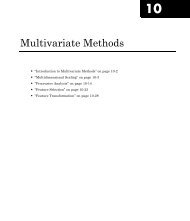
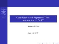
Examples That Use Standard AlgorithmsThis section presents the following examples:• “Simulink Example Using lsqnonlin” on page 2-27• “Simulink Example Using fminimax” on page 2-33• “Signal Processing Example” on page 2-36Simulink Example Using lsqnonlinSuppose that you want to optimize the control parameters in the Simulinkmodel optsim.mdl. (This model can be found in Optimization Toolbox optimdirectory. Note that Simulink must be installed on your system to load thismodel.) The model includes a nonlinear process plant modeled as a Simulinkblock diagram shown in Plant with Actuator Saturation on page 2-27.Plant with Actuator SaturationThe plant is an under-damped third-order model with actuator limits. Theactuator limits are a saturation limit and a slew rate limit. The actuatorsaturationlimitcutsoffinputvalues greater than 2 units or less than -2units. The slew rate limit of the actuator is 0.8 units/sec. The closed-loopresponse of the system to a step input is shown in Closed-Loop Response onpage 2-28. You can see this response by opening the model (type optsim atthe command line or click the model name), and selecting Start from theSimulation menu. The response plots to the scope.2-27

2 TutorialClosed-Loop ResponseThe problem is to design a feedback control loop that tracks a unit step inputto the system. The closed-loop plant is entered in terms of the blocks wherethe plant and actuator have been placed in a hierarchical Subsystem block.A Scope block displays output trajectories during the design process. SeeClosed-Loop Model on page 2-28.Closed-Loop Model2-28

Examples That Use Standard AlgorithmsOnewaytosolvethisproblemistominimizetheerrorbetweentheoutputand the input signal. The variables are the parameters of the ProportionalIntegral Derivative (PID) controller. If you only need to minimize the errorat one time unit, it would be a single objective function. But the goal isto minimize the error for all time steps from 0 to 100, thus producing amultiobjective function (one function for each time step).The routine lsqnonlin is used to perform a least-squares fit on the trackingoftheoutput. Thetrackingisperformed via an M-file function tracklsq,which returns the error signal yout, the output computed by calling sim,minus the input signal 1. Thecodefortracklsq, shown below, is contained inthe file runtracklsq.m, which is included in Optimization Toolbox.The function runtracklsq sets up all the needed values and then callslsqnonlin with the objective function tracklsq, which is nested insideruntracklsq. The variable options passed to lsqnonlin defines thecriteria and display characteristics. In this case you ask for output, use themedium-scale algorithm, and give termination tolerances for the step andobjective function on the order of 0.001.To run the simulation in the model optsim, thevariablesKp, Ki, Kd, a1, anda2 (a1 and a2 are variables in the Plant block) must all be defined. Kp, Ki, andKd are the variables to be optimized. The function tracklsq is nested insideruntracklsq so that the variables a1 and a2 aresharedbetweenthetwofunctions. The variables a1 and a2 are initialized in runtracklsq.The objective function tracklsq must run the simulation. The simulation canbe run either in the base workspace or the current workspace, that is, theworkspace of the function calling sim, which in this case is the workspace oftracklsq. In this example, the simset command is used to tell sim to run thesimulation in the current workspace by setting 'SrcWorkspace' to 'Current'.You can also choose a solver for sim using the simset function. The simulationis performed using a fixed-step fifth-order method to 100 seconds.When the simulation is completed, the variables tout, xout, andyout are nowin the current workspace (that is, the workspace of tracklsq). The Outportblock in the block diagram model puts yout into the current workspace at theend of the simulation.The following is the code for runtracklsq:2-29

2 Tutorialfunction [Kp,Ki,Kd] = runtracklsq% RUNTRACKLSQ demonstrates using LSQNONLIN with Simulink.optsim% Load the modelpid0 = [0.63 0.0504 1.9688]; % Set initial valuesa1 = 3; a2 = 43;% Initialize model plant variablesoptions = optimset('LargeScale','off','Display','iter',...'TolX',0.001,'TolFun',0.001);pid = lsqnonlin(@tracklsq, pid0, [], [], options);Kp = pid(1); Ki = pid(2); Kd = pid(3);function F = tracklsq(pid)% Track the output of optsim to a signal of 1% Variables a1 and a2 are needed by the model optsim.% They are shared with RUNTRACKLSQ so do not need to be% redefined here.Kp = pid(1);Ki = pid(2);Kd = pid(3);% Compute function valuesimopt = simset('solver','ode5',...'SrcWorkspace','Current');% Initialize sim options[tout,xout,yout] = sim('optsim',[0 100],simopt);F = yout-1;endendWhen you run runtracklsq, the optimization gives the solution for theproportional, integral, and derivative (Kp, Ki, Kd) gains of the controller after64 function evaluations.[Kp, Ki, Kd] = runtracklsqDirectionalIteration Func-count Residual Step-size derivative Lambda0 4 8.665312-30

Examples That Use Standard Algorithms1 18 5.21604 85.4 -0.00836 6.924692 25 4.53699 1 -0.107 0.04030593 32 4.47316 0.973 -0.00209 0.01343484 40 4.46854 2.45 9.72e-005 0.006762295 47 4.46575 0.415 -0.00266 0.003381156 48 4.46526 1 -0.000999 0.00184785Optimization terminated: directional derivative alongsearch direction less than TolFun and infinity-norm ofgradient less than 10*(TolFun+TolX).Kp =3.0956Ki =0.1466Kd =14.13782-31

2 TutorialThe resulting closed-loop step response is shown in Closed-Loop ResponseUsing lsqnonlin on page 2-32.Closed-Loop Response Using lsqnonlin2-32

Examples That Use Standard AlgorithmsNote The call to sim results in a call to one of the Simulink ordinarydifferential equation (ODE) solvers. A choice must be made about the type ofsolver to use. From the optimization point of view, a fixed-step solver is thebest choice if that is sufficient to solve the ODE. However, in the case of a stiffsystem,avariable-stepmethodmight be required to solve the ODE.The numerical solution produced by a variable-step solver, however, is not asmooth function of parameters, because of step-size control mechanisms. Thislack of smoothness can prevent the optimization routine from converging. Thelack of smoothness is not introduced when a fixed-step solver is used. (For afurther explanation, see [1].)The Simulink Response Optimization is recommended for solvingmultiobjective optimization problems in conjunction with variable-step solversin Simulink. It provides a special numeric gradient computation that workswith Simulink and avoids introducing a problem of lack of smoothness.Simulink Example Using fminimaxAnother approach to optimizing the control parameters in the Simulink modelshowninPlantwithActuator Saturation on page 2-27 is to use the fminimaxfunction. In this case, rather than minimizing the error between the outputand the input signal, you minimize the maximum value of the output at anytime t between 0 and 100.The code for this example, shown below, is contained in the functionruntrackmm, in which the objective function is simply the output youtreturned by the sim command. But minimizing the maximum output at alltimestepsmightforcetheoutputtobefarbelowunityforsometimesteps.To keep the output above 0.95 after the first 20 seconds, the constraintfunction trackmmcon contains the constraint yout >= 0.95 from t=20 tot=100. Because constraints must be in the form g

2 Tutorialcalling the simulation twice by using nested functions so that the value ofyout can be shared between the objective and constraint functions as long asit is initialized in runtrackmm.Thefollowingisthecodeforruntrackmm:function [Kp, Ki, Kd] = runtrackmmoptsimpid0 = [0.63 0.0504 1.9688];% a1, a2, yout are shared with TRACKMMOBJ and TRACKMMCONa1 = 3; a2 = 43; % Initialize plant variables in modelyout = []; % Give yout an initial valueoptions = optimset('Display','iter',...'TolX',0.001,'TolFun',0.001);pid = fminimax(@trackmmobj,pid0,[],[],[],[],[],[],...@trackmmcon,options);Kp = pid(1); Ki = pid(2); Kd = pid(3);function F = trackmmobj(pid)% Track the output of optsim to a signal of 1.% Variables a1 and a2 are shared with RUNTRACKMM.% Variable yout is shared with RUNTRACKMM and% RUNTRACKMMCON.endKp = pid(1);Ki = pid(2);Kd = pid(3);% Compute function valueopt = simset('solver','ode5','SrcWorkspace','Current');[tout,xout,yout] = sim('optsim',[0 100],opt);F = yout;function [c,ceq] = trackmmcon(pid)% Track the output of optsim to a signal of 1.% Variable yout is shared with RUNTRACKMM and% TRACKMMOBJ2-34

Examples That Use Standard Algorithmsendend% Compute constraints.% Objective TRACKMMOBJ is called before this% constraint function, so yout is current.c = -yout(20:100)+.95;ceq=[];When you run the code, it returns the following results:[Kp,Ki,Kd] = runtrackmmMaxDirectionalIter F-count {F,constraints} Step-size derivative Procedure0 5 1.119821 11 1.264 1 1.182 17 1.055 1 -0.1723 23 1.004 1 -0.0128 Hessian modified twice4 29 0.9997 1 3.48e-005 Hessian modified5 35 0.9996 1 -1.36e-006 Hessian modified twiceOptimization terminated: magnitude of directional derivative in searchdirection less than 2*options.TolFun and maximum constraint violationis less than options.TolCon.lower upper ineqlin ineqnonlin114182Kp =0.5894Ki =0.0605Kd =5.52952-35

2 TutorialThe last value shown in the MAX{F,constraints} column of the output showsthat the maximum value for all the time steps is 0.9996. The closed loopresponse with this result is shown in the following Closed-Loop ResponseUsing fminimax on page 2-36.This solution differs from the solution lsqnonlin because you are solvingdifferent problem formulations.Closed-Loop Response Using fminimaxSignal Processing ExampleConsider designing a linear-phase Finite Impulse Response (FIR) filter. Theproblem is to design a lowpass filter with magnitude one at all frequenciesbetween 0 and 0.1 Hz and magnitude zero between 0.15 and 0.5 Hz.The frequency response H(f) for such a filter is defined by2-36

Examples That Use Standard Algorithms(2-6)where A(f) isthe magnitude of the frequency response. One solution is toapply a goal attainment method to the magnitude of the frequency response.Given a function that computes the magnitude, the function fgoalattainwill attempt to varythemagnitudecoefficientsa(n) until the magnituderesponse matches the desired response within some tolerance. The functionthat computes the magnitude response is given in filtmin.m. This functiontakes a, themagnitude function coefficients, and w, the discretization of thefrequency domain we are interested in.To set up a goal attainment problem, you must specify the goal and weightsfor the problem. For frequencies between 0 and 0.1, the goal is one. Forfrequencies between 0.15 and 0.5, the goal is zero. Frequencies between 0.1and 0.15 are not specified, so no goals or weights are needed in this range.This information is stored in the variable goal passed to fgoalattain.The length of goal is the same as the length returned by the functionfiltmin. So that the goals are equally satisfied, usually weight wouldbe set to abs(goal). However, since some of the goals are zero, the effectof using weight=abs(goal) will force the objectives with weight 0tobesatisfied as hard constraints, and the objectives with weight 1 possibly to beunderattained (see “Goal Attainment Method” on page 3-49). Because all thegoals are close in magnitude, using a weight of unity for all goals will givethem equal priority. (Using abs(goal) for the weights is more importantwhen the magnitude of goal differs more significantly.) Also, settingoptions = optimset('GoalsExactAchieve',length(goal));specifies that each objective should be as nearaspossibletoitsgoalvalue(neither greater nor less than).2-37

2 TutorialStep 1: Write an M-file filtmin.m.function y = filtmin(a,w)n = length(a);y = cos(w'*(0:n-1)*2*pi)*a ;Step 2: Invoke optimization routine.% Plot with initial coefficientsa0 = ones(15,1);incr = 50;w = linspace(0,0.5,incr);y0 = filtmin(a0,w);clf, plot(w,y0,'.r');drawnow;% Set up the goal attainment problemw1 = linspace(0,0.1,incr) ;w2 = linspace(0.15,0.5,incr);w0 = [w1 w2];goal = [1.0*ones(1,length(w1)) zeros(1,length(w2))];weight = ones(size(goal));% Call fgoalattainoptions = optimset('GoalsExactAchieve',length(goal));[a,fval,attainfactor,exitflag]=fgoalattain(@(x) filtmin(x,w0)...a0,goal,weight,[],[],[],[],[],[],[],options);% Plot with the optimized (final) coefficientsy = filtmin(a,w);hold on, plot(w,y,'r')axis([0 0.5 -3 3])xlabel('Frequency (Hz)')ylabel('Magnitude Response (dB)')legend('initial', 'final')grid on2-38

Examples That Use Standard AlgorithmsCompare the magnitude response computed with the initial coefficients andthe final coefficients (Magnitude Response with Initial and Final MagnitudeCoefficients on page 2-39). Note that you could use the firpm function in theSignal Processing Toolbox to design this filter.Magnitude Response with Initial and Final Magnitude Coefficients2-39

2 TutorialLarge-Scale Examples• “Introduction” on page 2-40• “Problems Covered by Large-Scale Methods” on page 2-41• “Nonlinear Equations with Jacobian” on page 2-45• “Nonlinear Equations with Jacobian Sparsity Pattern” on page 2-47• “Nonlinear Least-Squares with Full Jacobian Sparsity Pattern” on page2-50• “Nonlinear Minimization with Gradient and Hessian” on page 2-51• “Nonlinear Minimization with Gradient and Hessian Sparsity Pattern”on page 2-53• “Nonlinear Minimization with Bound Constraints and BandedPreconditioner” on page 2-55• “Nonlinear Minimization with Equality Constraints” on page 2-59• “Nonlinear Minimization with a Dense but Structured Hessian andEquality Constraints” on page 2-61• “Quadratic Minimization with Bound Constraints” on page 2-65• “Quadratic Minimization with a Dense but Structured Hessian” on page2-67• “Linear Least-Squares with Bound Constraints” on page 2-72• “Linear Programming with Equalities and Inequalities” on page 2-73• “Linear Programming with Dense Columns in the Equalities” on page 2-75IntroductionSome of the optimization functions include algorithms for continuousoptimization problems especially targeted to large problems with sparsity orstructure. The main large-scale algorithms are iterative, i.e., a sequenceof approximate solutions is generated. In each iteration a linear system is(approximately) solved. The linear systems are solved using the sparse matrixcapabilities of MATLAB and a variety of sparse linear solution techniques,both iterative and direct.2-40

Large-Scale ExamplesGenerally speaking, the large-scale optimization methods preserve structureand sparsity, using exact derivative information wherever possible. To solvethe large-scale problems efficiently, some problem formulations are restricted(such as only solving overdetermined linear or nonlinear systems), or requireadditional information (e.g., the nonlinear minimization algorithm requiresthat the gradient be computed in the user-supplied function).This section summarizes the kinds of problems covered by large-scale methodsand provides examples.Problems Covered by Large-Scale MethodsThis section describes how to formulate problems for functions that uselarge-scale methods. It is important to keep in mind that there are somerestrictions on the types of problems covered by large-scale methods. Forexample, the function fmincon cannot use large-scale methods when thefeasible region is defined by either of the following:• Nonlinear equality or inequality constraints• Both upper- or lower-bound constraints and equality constraintsWhen a function is unable to solve a problem using large-scale methods, itreverts to medium-scale methods.Formulating Problems with Large-Scale MethodsThefollowingtablesummarizeshowto set up problems for large-scalemethods and provide the necessary input for the optimization functions. Foreach function, the second column of the table describes how to formulatethe problem and the third column describes what additional information isneeded for the large-scale algorithms. For fminunc and fmincon, the gradientmust be computed along with the objective in the user-supplied function (thegradient is not required for the medium-scale algorithms).Since these methods can also be used on small- to medium-scale problemsthat are not necessarily sparse, the lastcolumnofthetableemphasizeswhatconditions are needed for large-scale problems to run efficiently withoutexceeding your computer system’s memory capabilities, e.g., the linearconstraint matrices should be sparse. For smaller problems the conditionsin the last column are unnecessary.2-41

2 TutorialNote The following table lists the functions in order of increasing problemcomplexity.Several examples, which follow this table, clarify the contents of the table.Large-Scale Problem Coverage and RequirementsFunctionProblemFormulationsAdditionalInformationNeededFor Large ProblemsfminuncMust providegradient forf(x) in fun.• Provide sparsitystructure of the Hessian,or compute the Hessianin fun.• The Hessian should besparse.fmincon•such that where .•such that,andis an m-by-n matrixwhereMust providegradient forf(x) in fun.• Provide sparsitystructure of the Hessianor compute the Hessianin fun.• The Hessian should besparse.• should be sparse.2-42

Large-Scale ExamplesLarge-Scale Problem Coverage and Requirements (Continued)FunctionProblemFormulationsAdditionalInformationNeededFor Large Problemslsqnonlin••such that where .None• Provide sparsitystructure of the Jacobianor compute the Jacobianin fun.• The Jacobian should besparse.F(x) must be overdetermined(have at least as many equationsas variables).lsqcurvefit••such thatwhereNone• Provide sparsitystructure of the Jacobianor compute the Jacobianin fun.• The Jacobian should besparse.must beoverdetermined (have at least asmany equations as variables).fsolvemust have the samenumber of equations asvariables.None• Provide sparsitystructure of the Jacobianor compute the Jacobianin fun.• The Jacobian should besparse.2-43

2 TutorialLarge-Scale Problem Coverage and Requirements (Continued)FunctionProblemFormulationsAdditionalInformationNeededFor Large ProblemslsqlinNoneshould be sparse.linprogsuch that where .is an m-by-n matrix wherei.e., the problem must beoverdetermined.None and should be sparse.such thatand,where .quadprog•such thatwhereNone • should be sparse.• should be sparse.•such that,andis an m-by-n matrixwhereIn the following examples, many of the M-file functions are available inOptimization Toolbox optim directory. Most of these do not have a fixedproblem size, i.e., the size of your starting point xstart determines the sizeproblem that is computed. If your computer system cannot handle the sizesuggested in the examples below, use a smaller-dimension start point to runtheproblems.Iftheproblemshaveupper or lower bounds or equalities, youmust adjust the size of those vectors or matrices as well.2-44

Large-Scale ExamplesNonlinear Equations with JacobianConsider the problem of finding a solution to a system of nonlinear equationswhose Jacobian is sparse. The dimension of the problem in this exampleis 1000. The goal is to find x such that F(x) =0. Assumingn = 1000, thenonlinear equations areTo solve a large nonlinear system of equations, F(x) = 0, use the large-scalemethod available in fsolve.Step 1: Write an M-file nlsf1.m that computes the objectivefunction values and the Jacobian.function [F,J] = nlsf1(x);% Evaluate the vector functionn = length(x);F = zeros(n,1);i = 2:(n-1);F(i) = (3-2*x(i)).*x(i)-x(i-1)-2*x(i+1)1+ 1;F(n) = (3-2*x(n)).*x(n)-x(n-1) + 1;F(1) = (3-2*x(1)).*x(1)-2*x(2) + 1;% Evaluate the Jacobian if nargout > 1if nargout > 1d = -4*x + 3*ones(n,1); D = sparse(1:n,1:n,d,n,n);c = -2*ones(n-1,1); C = sparse(1:n-1,2:n,c,n,n);e = -ones(n-1,1); E = sparse(2:n,1:n-1,e,n,n);J = C + D + E;endStep 2: Call the solve routine for the system of equations.xstart = -ones(1000,1);fun = @nlsf1;options =2-45

2 Tutorialoptimset('Display','iter','LargeScale','on','Jacobian','on');[x,fval,exitflag,output] = fsolve(fun,xstart,options);A starting point is given as well as the function name. The default method forfsolve is medium-scale, so it is necessary to specify 'LargeScale' as 'on' inthe options argument. Setting the Display option to 'iter' causes fsolveto display the output at each iteration. Setting Jacobian to 'on', causesfsolve to use the Jacobian information available in nlsf1.m.The commands display this output:Norm of First-order CG-Iteration Func-count f(x) step optimality Iterations1 2 1011 1 19 02 3 16.1942 7.91898 2.35 33 4 0.0228027 1.33142 0.291 34 5 0.000103359 0.0433329 0.0201 45 6 7.3792e-007 0.0022606 0.000946 46 7 4.02299e-010 0.000268381 4.12e-005 5Optimization terminated successfully:Relative function value changing by less than OPTIONS.TolFunA linear system is (approximately) solved in each major iteration usingthe preconditioned conjugate gradient method. The default value forPrecondBandWidth is 0 in options, so a diagonal preconditioner is used.(PrecondBandWidth specifies the bandwidth of the preconditioning matrix. Abandwidth of 0 means there is only one diagonal in the matrix.)From the first-order optimality values, fast linear convergence occurs. Thenumber of conjugate gradient (CG) iterations required per major iteration islow, at most five for a problem of 1000 dimensions, implying that the linearsystems are not very difficult to solve in this case (though more work isrequired as convergence progresses).It is possible to override the default choice of preconditioner (diagonal)by choosing a banded preconditioner through the use of the optionPrecondBandWidth. If you want to use a tridiagonal preconditioner, i.e.,a preconditioning matrix with three diagonals (or bandwidth of one), setPrecondBandWidth to the value 1:options = optimset('Display','iter','Jacobian','on',...2-46

Large-Scale Examples'LargeScale','on','PrecondBandWidth',1);[x,fval,exitflag,output] = fsolve(fun,xstart,options);In this case the output isNorm of First-order CG-Iteration Func-count f(x) step optimality Iterations1 2 1011 1 19 02 3 16.0839 7.92496 1.92 13 4 0.0458181 1.3279 0.579 14 5 0.000101184 0.0631898 0.0203 25 6 3.16615e-007 0.00273698 0.00079 26 7 9.72481e-010 0.00018111 5.82e-005 2Optimization terminated successfully:Relative function value changing by less than OPTIONS.TolFunNote that although the same number of iterations takes place, the numberof PCG iterations has dropped, so less work is being done per iteration. See“Preconditioned Conjugate Gradients” on page 4-7.Nonlinear Equations with Jacobian Sparsity PatternIn the preceding example, the function nlsf1 computes the Jacobian J, asparse matrix, along with the evaluation of F. What if the code to compute theJacobian is not available? By default, if you do not indicate that the Jacobiancan be computed in nlsf1 (by setting the Jacobian option in options to'on'), fsolve, lsqnonlin, andlsqcurvefit instead uses finite differencingto approximate the Jacobian.In order for this finite differencing to be as efficient as possible, you shouldsupply the sparsity pattern of the Jacobian, by setting JacobPattern to 'on'in options. That is, supply a sparse matrix Jstr whose nonzero entriescorrespond to nonzeros of the Jacobian for all x. Indeed,thenonzerosofJstrcan correspond to a superset of the nonzero locations of J; however, in generalthe computational cost of the sparse finite-difference procedure will increasewith the number of nonzeros of Jstr.Providing the sparsity pattern can drastically reduce the time needed tocompute the finite differencing on large problems. If the sparsity patternis not provided (and the Jacobian is not computed in the objective function2-47

2 Tutorialeither) then, in this problem nlsfs1, the finite-differencing code attempts tocompute all 1000-by-1000 entries in the Jacobian. But in this case there areonly 2998 nonzeros, substantially less than the 1,000,000 possible nonzerosthe finite-differencing code attempts to compute. In other words, this problemis solvable if you provide the sparsity pattern. If not, most computers run outof memory when the full dense finite-differencing is attempted. On mostsmall problems, it is not essential to provide the sparsity structure.SupposethesparsematrixJstr, computed previously, has been saved in filenlsdat1.mat. The following driver calls fsolve applied to nlsf1a, whichisthesameasnlsf1 except that only the function values are returned; sparsefinite-differencing is used to estimate the sparse Jacobian matrix as needed.Step 1: Write an M-file nlsf1a.m that computes the objectivefunction values.function F = nlsf1a(x);% Evaluate the vector functionn = length(x);F = zeros(n,1);i = 2:(n-1);F(i) = (3-2*x(i)).*x(i)-x(i-1)-2*x(i+1) + 1;F(n) = (3-2*x(n)).*x(n)-x(n-1) + 1;F(1) = (3-2*x(1)).*x(1)-2*x(2) + 1;Step 2: Call the system of equations solve routine.xstart = -ones(1000,1);fun = @nlsf1a;load nlsdat1 % Get Jstroptions = optimset('Display','iter','JacobPattern',Jstr,...'LargeScale','on','PrecondBandWidth',1);[x,fval,exitflag,output] = fsolve(fun,xstart,options);In this case, the output displayed isNorm of First-order CG-Iteration Func-count f(x) step optimality Iterations1 6 1011 1 19 02 11 16.0839 7.92496 1.92 12-48

Large-Scale Examples3 16 0.0458181 1.3279 0.579 14 21 0.000101184 0.0631898 0.0203 25 26 3.16615e-007 0.00273698 0.00079 26 31 9.72482e-010 0.00018111 5.82e-005 2Optimization terminated successfully:Relative function value changing by less than OPTIONS.TolFunAlternatively, it is possible to choose a sparse direct linear solver (i.e., a sparseQR factorization) by indicating a “complete” preconditioner. For example, ifyou set PrecondBandWidth to Inf, then a sparse direct linear solver is usedinstead of a preconditioned conjugate gradient iteration:xstart = -ones(1000,1);fun = @nlsf1a;load nlsdat1 % Get Jstroptions = optimset('Display','iter','JacobPattern',Jstr,...'LargeScale','on','PrecondBandWidth',inf);[x,fval,exitflag,output] = fsolve(fun,xstart,options);and the resulting display isNorm of First-order CG-Iteration Func-count f(x) step optimality Iterations1 6 1011 1 19 02 11 15.9018 7.92421 1.89 13 16 0.0128163 1.32542 0.0746 14 21 1.73538e-008 0.0397925 0.000196 15 26 1.13169e-018 4.55544e-005 2.76e-009 1Optimization terminated successfully:Relative function value changing by less than OPTIONS.TolFunWhenthesparsedirectsolversareused,theCGiterationis1forthat(major)iteration, as shown in the output under CG-Iterations. Notice that the finaloptimality and f(x) value (which for fsolve, f(x), is the sum of the squares ofthe function values) are closer to zero than using the PCG method, whichis often the case.2-49

2 TutorialNonlinear Least-Squares with Full Jacobian SparsityPatternThe large-scale methods in lsqnonlin, lsqcurvefit, andfsolve can be usedwith small- to medium-scale problems without computing the Jacobian in funor providing the Jacobiansparsitypattern.(Thisexamplealsoappliestothecase of using fmincon or fminunc without computing the Hessian or supplyingthe Hessian sparsity pattern.) How small is small- to medium-scale? Noabsolute answer is available, as it depends on the amount of virtual memoryavailable in yourcomputersystemconfiguration.Suppose your problem has m equations and n unknowns. If the commandJ = sparse(ones(m,n)) causes an Out of memory error on your machine,then this is certainly too large a problem. If it does not result in an error,the problem might still be too large, but you can only find out by running itand seeing if MATLABisabletorunwithintheamountofvirtualmemoryavailable on yoursystem.Let’s say you have a small problem with 10 equations and 2 unknowns, suchas finding x that minimizesstarting at the point x = [0.3, 0.4].Because lsqnonlin assumes that the sum of squares is not explicitly formedin the user function, the function passed to lsqnonlin should instead computethe vector valued functionfor(that is,F should have 10 components).Step 1: Write an M-file myfun.m that computes the objectivefunction values.function F = myfun(x)k = 1:10;2-50

Large-Scale ExamplesF = 2 + 2*k-exp(k*x(1))-exp(k*x(2));Step 2: Call the nonlinear least-squares routine.x0 = [0.3 0.4]% Starting guess[x,resnorm] = lsqnonlin(@myfun,x0) % Invoke optimizerBecause the Jacobian is not computed in myfun.m, and no Jacobiansparsity pattern is provided by the JacobPattern option in options,lsqnonlin calls the large-scale method with JacobPattern set toJstr = sparse(ones(10,2)). Thisisthedefaultforlsqnonlin. Notethatthe Jacobian option in options is set to 'off' by default.When the finite-differencing routine is called the first time, it detects thatJstr is actually a dense matrix, i.e., that no speed benefit is derived fromstoring it as a sparse matrix. From then on the finite-differencing routineuses Jstr = ones(10,2) (a full matrix) for the optimization computations.After about 24 function evaluations, this example gives the solutionx =0.2578 0.2578resnorm % Residual or sum of squaresresnorm =124.3622Most computer systems can handle much larger full problems, say into the100s of equations and variables. But if there is some sparsity structure in theJacobian (or Hessian) that can be taken advantage of, the large-scale methodswill always run faster if this information is provided.Nonlinear Minimization with Gradient and HessianThis example involves solving a nonlinear minimization problem with atridiagonal Hessian matrix H(x) first computed explicitly, and then byproviding the Hessian’s sparsity structure for the finite-differencing routine.2-51

2 TutorialThe problem is to find x to minimize(2-7)where n = 1000.Step 1: Write an M-file brownfgh.m that computes theobjective function, the gradient of the objective, and the sparsetridiagonal Hessian matrix.This file is rather long and is not included here. You can view the code withthe commandtype brownfghBecause brownfgh computes the gradient and Hessian values as well as theobjective function, you need to use optimset to indicate that this informationis available in brownfgh, usingtheGradObj and Hessian options.Step 2: Call a nonlinear minimization routine with a startingpoint xstart.n = 1000;xstart = -ones(n,1);xstart(2:2:n,1) = 1;options = optimset('GradObj','on','Hessian','on');[x,fval,exitflag,output] = fminunc(@brownfgh,xstart,options);This 1000 variable problem is solved in about 7 iterations and 7 conjugategradient iterations with a positive exitflag indicating convergence. Thefinal function value and measure of optimality at the solution x are both closeto zero. For fminunc, the first order optimality is the infinity norm of thegradient of the function, which is zero at a local minimum:exitflag =1fval =2.8709e-017output.iterations2-52

2 Tutoriali=1:(n-1); g = zeros(n,1);g(i) = 2*(x(i+1).^2+1).*x(i).* ...((x(i).^2).^(x(i+1).^2))+ ...2*x(i).*((x(i+1).^2).^(x(i).^2+1)).* ...log(x(i+1).^2);g(i+1) = g(i+1) + ...2*x(i+1).*((x(i).^2).^(x(i+1).^2+1)).* ...log(x(i).^2) + ...2*(x(i).^2+1).*x(i+1).* ...((x(i+1).^2).^(x(i).^2));endTo allow efficient computation of the sparse finite-difference approximation ofthe Hessian matrix H(x), the sparsity structure of H must be predetermined.In this case assume this structure, Hstr, a sparse matrix, is available in filebrownhstr.mat. Usingthe spy command you can see that Hstr is indeedsparse (only 2998 nonzeros). Use optimset to set the HessPattern optionto Hstr. When a problem as large as this has obvious sparsity structure,not setting the HessPattern option requires a huge amount of unnecessarymemory and computation because fminunc attempts to use finite differencingon a full Hessian matrix of one million nonzero entries.You must also set the GradObj option to 'on' using optimset, sincethegradient is computed in brownfg.m. Thenexecutefminunc asshowninStep2.Step 2: Call a nonlinear minimization routine with a startingpoint xstart.fun = @brownfg;load brownhstr% Get Hstr, structure of the Hessianspy(Hstr)% View the sparsity structure of Hstrn = 1000;xstart = -ones(n,1);xstart(2:2:n,1) = 1;options = optimset('GradObj','on','HessPattern',Hstr);[x,fval,exitflag,output] = fminunc(fun,xstart,options);This 1000-variable problem is solved in eight iterations and seven conjugategradient iterations with a positive exitflag indicating convergence. Thefinal function value and measure of optimality at the solution x are both close2-54

Large-Scale Examplesto zero (for fminunc, the first-order optimality is the infinity norm of thegradient of the function, which is zero at a local minimum):exitflag =1fval =7.4739e-017output.iterationsans =7output.cgiterationsans =7output.firstorderoptans =7.9822e-010Nonlinear Minimization with Bound Constraints andBanded PreconditionerThe goal in this problem is to minimize the nonlinear functionsuch that ,wheren is 800 (n should be a multiple of 4),,and .Step 1: Write an M-file tbroyfg.m that computes the objectivefunction and the gradient of the objectiveThe M-file function tbroyfg.m computes the function value and gradient.This file is long and is not included here. You can see the code for this functionusing the commandtype tbroyfg2-55

2 TutorialThe sparsity pattern of the Hessian matrix has been predetermined andstored in the file tbroyhstr.mat. The sparsity structure for the Hessian ofthis problem is banded, as you can see in the following spy plot.load tbroyhstrspy(Hstr)01002003004005006007008000 100 200 300 400 500 600 700 800nz = 4794In this plot, the center stripe is itself a five-banded matrix. The followingplot shows the matrix more clearly:spy(Hstr(1:20,1:20))2-56

Large-Scale Examples024681012141618200 2 4 6 8 10 12 14 16 18 20nz = 94Use optimset to set the HessPattern parameter to Hstr. Whenaproblemaslargeasthishasobvioussparsitystructure,notsettingtheHessPatternparameter requires a huge amount of unnecessary memory and computation.This is because fmincon attempts to use finite differencing on a full Hessianmatrix of 640,000 nonzero entries.You must also set the GradObj parameter to 'on' using optimset, sincethegradient is computed in tbroyfg.m. Thenexecutefmincon asshowninStep2.Step 2: Call a nonlinear minimization routine with a startingpoint xstart.fun = @tbroyfg;load tbroyhstr% Get Hstr, structure of the Hessiann = 800;xstart = -ones(n,1); xstart(2:2:n) = 1;lb = -10*ones(n,1); ub = -lb;options = optimset('GradObj','on','HessPattern',Hstr);[x,fval,exitflag,output] = ...fmincon(fun,xstart,[],[],[],[],lb,ub,[],options);After seven iterations, the exitflag, fval, andoutput values are2-57

2 Tutorialexitflag =3fval =270.4790output =iterations: 7funcCount: 8cgiterations: 18firstorderopt: 0.0163algorithm: 'large-scale: trust-region reflective Newton'message: [1x86 char]For bound constrained problems, the first-order optimality is the infinitynorm of v.*g, wherev is defined as in “Box Constraints” on page 4-10, and gis the gradient.Because of the five-banded center stripe, you can improve the solutionby using a five-banded preconditioner instead of the default diagonalpreconditioner. Using the optimset function, reset the PrecondBandWidthparameter to 2 and solve the problem again. (The bandwidth is the number ofupper (or lower) diagonals, not counting the main diagonal.)fun = @tbroyfg;load tbroyhstr% Get Hstr, structure of the Hessiann = 800;xstart = -ones(n,1); xstart(2:2:n,1) = 1;lb = -10*ones(n,1); ub = -lb;options = optimset('GradObj','on','HessPattern',Hstr, ...'PrecondBandWidth',2);[x,fval,exitflag,output] = ...fmincon(fun,xstart,[],[],[],[],lb,ub,[],options);The number of iterations actually goes up by two; however the total numberof CG iterations drops from 18 to 15. The first-order optimality measure isreduced by a factor of 1e-3:exitflag =32-58

Large-Scale Examplesfval =270.4790output =iterations: 9funcCount: 10cgiterations: 15firstorderopt: 7.5340e-005algorithm: 'large-scale: trust-region reflective Newton'message: [1x86 char]Nonlinear Minimization with Equality ConstraintsThe large-scale method for fmincon can handle equality constraints if noother constraints exist. Suppose you want to minimize the same objectiveas in Equation 2-7, which is coded in the function brownfgh.m, wheren =1000, such that for Aeq that has 100 equations (so Aeq is a100-by-1000 matrix).Step 1: Write an M-file brownfgh.m that computes theobjective function, the gradient of the objective, and the sparsetridiagonal Hessian matrix.As before, this file is rather long and is not included here. You can view thecode with the commandtype brownfghBecause brownfgh computes the gradient and Hessian values as well as theobjective function, you need to use optimset to indicate that this informationis available in brownfgh, usingtheGradObj and Hessian options.ThesparsematrixAeq and vector beq are available in the file browneq.mat:load browneqThe linear constraint system is 100-by-1000, has unstructured sparsity (usespy(Aeq) to view the sparsity structure), and is not too badly ill-conditioned:condest(Aeq*Aeq')ans =2-59

2 Tutorial2.9310e+006Step 2: Call a nonlinear minimization routine with a startingpoint xstart.fun = @brownfgh;load browneq% Get Aeq and beq, the linear equalitiesn = 1000;xstart = -ones(n,1); xstart(2:2:n) = 1;options = optimset('GradObj','on','Hessian','on', ...'PrecondBandWidth', inf);[x,fval,exitflag,output] = ...fmincon(fun,xstart,[],[],Aeq,beq,[],[],[],options);Setting the option PrecondBandWidth to inf causes a sparse direct solver tobe used instead of preconditioned conjugate gradients.The exitflag value of 3 indicates that the algorithm terminated because thechange in the objective function value was less than the specified toleranceTolFun. The final function value is given by fval.exitflag =3fval =205.9313output =iterations: 16funcCount: 17cgiterations: 20firstorderopt: 7.3575e-005algorithm: 'large-scale: projected trust-region Newton'message: [1x86 char]The linear equalities are satisfied at x.norm(Aeq*x-beq)2-60

Large-Scale Examplesans =1.1885e-012Nonlinear Minimization with a Dense but StructuredHessian and Equality ConstraintsThe fmincon and fminunc large-scale methods can solve problems where theHessian is dense but structured. For these problems, fmincon and fminunc donot compute H*Y with the Hessian H directly, as they do for medium-scaleproblems and for large-scale problems with sparse H, becauseformingHwould be memory-intensive. Instead, you must provide fmincon or fminuncwith a function that, given a matrix Y and information about H, computesW = H*Y.In this example, the objective function is nonlinear and linear equalities existso fmincon is used. The objective function has the structurewhere V is a 1000-by-2 matrix. The Hessian of f is dense, but the Hessian ofis sparse. If the Hessian of is ,then ,theHessianof ,isTo avoid excessive memory usage that could happen by working with Hdirectly, the example provides a Hessian multiply function, hmfleq1. Thisfunction, when passed a matrix Y, uses sparse matrices Hinfo, whichcorresponds to ,andV to compute the Hessian matrix productW = H*Y = (Hinfo - V*V')*YIn this example, the Hessian multiply function needs and V to compute theHessian matrix product. V is a constant, so you can capture V in a functionhandle to an anonymous function.However, is not a constant and must be computed at the current x. Youcando this by computing in the objective function and returning as Hinfo inthe third output argument. By using optimset to set the 'Hessian' options2-61

2 Tutorialto 'on', fmincon knows to get the Hinfo value from the objective function andpass it to the Hessian multiply function hmfleq1.Step 1: Write an M-file brownvv.m that computes the objectivefunction, the gradient, and the sparse part of the Hessian.The example passes brownvv to fmincon as the objective function. Thebrownvv.m file is long and is not included here. You can view the code withthe commandtype brownvvBecause brownvv computes the gradient and part of the Hessian as well asthe objective function, the example (Step 3) uses optimset to set the GradObjand Hessian options to 'on'.Step 2: Write a function to compute Hessian-matrix productsfor H given a matrix Y.Now, define a function hmfleq1 that uses Hinfo, which is computedin brownvv, andV, which you can capture in a function handle to ananonymous function, to compute the Hessian matrix product W whereW = H*Y = (Hinfo - V*V')*Y. This function must have the formW = hmfleq1(Hinfo,Y)The first argument must be the same as the third argument returned by theobjective function brownvv. The second argument to the Hessian multiplyfunction is the matrix Y (of W = H*Y).Because fmincon expects the second argument Y to be used to form theHessian matrix product, Y is always a matrix with n rows where n is thenumber of dimensions in the problem. The number of columns in Y can vary.Finally, you can use a function handle to an anonymous function to captureV, so V can be the third argument to 'hmfleqq'.function W = hmfleq1(Hinfo,Y,V);%HMFLEQ1 Hessian-matrix product function for BROWNVV objective.% W = hmfleq1(Hinfo,Y,V) computes W = (Hinfo-V*V')*Y% where Hinfo is a sparse matrix computed by BROWNVV% and V is a 2 column matrix.2-62

Large-Scale ExamplesW = Hinfo*Y - V*(V'*Y);Note The function hmfleq1 is available in Optimization Toolbox as the M-filehmfleq1.m.Step 3: Call a nonlinear minimization routine with a startingpoint and linear equality constraints.Load the problem parameter, V, and the sparse equality constraint matrices,Aeq and beq, fromfleq1.mat, which is available in Optimization Toolbox.Use optimset to set the GradObj and Hessian options to 'on' and to set theHessMult option to a function handle that points to hmfleq1. Callfminconwith objective function brownvv and with V as an additional parameter:function [fval, exitflag, output, x] = runfleq1% RUNFLEQ1 demonstrates 'HessMult' option for% FMINCON with linear equalities.% Copyright 1984-2004 The MathWorks, Inc.% $Revision: 1.1.4.34.2.4 $ $Date: 2007/02/13 17:41:29 $problem = load('fleq1'); % Get V, Aeq, beqV = problem.V; Aeq = problem.Aeq; beq = problem.beq;n = 1000;% problem dimensionxstart = -ones(n,1); xstart(2:2:n,1) = ones(length(2:2:n),1);% starting pointoptions = optimset('GradObj','on','Hessian','on','HessMult',...@(Hinfo,Y)hmfleq1(Hinfo,Y,V) ,'Display','iter','TolFun',1e-9);[x,fval,exitflag,output] = fmincon(@(x)brownvv(x,V),...xstart,[],[],Aeq,beq,[],[], [],options);Note Type [fval,exitflag,output,x] = runfleq1; to run the precedingcode. This command displays the values for fval, exitflag, andoutput, aswell as the following iterative display.Because the iterative display was set using optimset, theresultsdisplayedare2-63

2 TutorialNorm of First-orderIteration f(x) step optimality CG-iterations1 1997.07 1 555 02 1072.56 6.31716 377 13 480.232 8.19554 159 24 136.861 10.3015 59.5 25 44.3708 9.04697 16.3 26 44.3708 100 16.3 27 44.3708 25 16.3 08 -8.90967 6.25 28.5 09 -318.486 12.5 107 110 -318.486 12.5 107 111 -415.445 3.125 73.9 012 -561.688 3.125 47.4 213 -785.326 6.25 126 314 -785.326 4.30584 126 515 -804.414 1.07646 26.9 016 -822.399 2.16965 2.8 317 -823.173 0.40754 1.34 318 -823.241 0.154885 0.555 319 -823.246 0.0518407 0.214 520 -823.246 0.00977601 0.00724 6Optimization terminated successfully:Relative function value changing by less than OPTIONS.TolFunConvergence is rapid for a problem of this size with the PCG iteration costincreasing modestly as the optimization progresses. Feasibility of the equalityconstraints is maintained at the solutionnorm(Aeq*x-beq)ans =1.9854e-013PreconditioningIn this example, fmincon cannot use H to compute a preconditioner because Honly exists implicitly. Instead of H, fmincon uses Hinfo, the third argumentreturned by brownvv, to compute a preconditioner. Hinfo is a good choicebecause it is the same size as H and approximates H to some degree. If Hinfo2-64

Large-Scale Exampleswere not the same size as H, fmincon would compute a preconditioner basedon some diagonal scaling matrices determined from the algorithm. Typically,this would not perform as well.Quadratic Minimization with Bound ConstraintsTo minimize a large-scale quadratic with upper and lower bounds, you canuse the quadprog function.The problem stored in the MAT-file qpbox1.mat is a positive definitequadratic, and the Hessian matrix H is tridiagonal, subject to upper (ub) andlower (lb) bounds.Step 1: Load the Hessian and define f, lb, and ub.load qpbox1 % Get Hlb = zeros(400,1); lb(400) = -inf;ub = 0.9*ones(400,1); ub(400) = inf;f = zeros(400,1); f([1 400]) = -2;Step 2: Call a quadratic minimization routine with a startingpoint xstart.xstart = 0.5*ones(400,1);[x,fval,exitflag,output] = ...quadprog(H,f,[],[],[],[],lb,ub,xstart);Looking at the resulting values of exitflag and output,exitflag =3output =iterations: 20algorithm: 'large-scale: reflective trust-region'firstorderopt: 9.6206e-006cgiterations: 1834message: [1x206 char]you can see that while convergence occurred in 20 iterations, the high numberof CG iterations indicates that the cost of the linear system solve is high. In2-65

2 Tutoriallight of this cost, one strategy would be to limit the number of CG iterationsper optimization iteration. The default number is the dimension of theproblem divided by two, 200 for this problem. Suppose you limit it to 50 usingthe MaxPCGIter flag in options:options = optimset('MaxPCGIter',50);[x,fval,exitflag,output] = ...quadprog(H,f,[],[],[],[],lb,ub,xstart,options);This time convergence still occurs and the total number of CG iterations(1547) has dropped:exitflag =3output =iterations: 36algorithm: 'large-scale: reflective trust-region'firstorderopt: 2.3821e-005cgiterations: 1547message: [1x206 char]A second strategy would be to use a direct solver at each iteration by settingthe PrecondBandWidth option to inf:options = optimset('PrecondBandWidth',inf);[x,fval,exitflag,output] = ...quadprog(H,f,[],[],[],[],lb,ub,xstart,options);Now the number of iterations has dropped to 10:exitflag =3output =iterations: 10algorithm: 'large-scale: reflective trust-region'firstorderopt: 1.2319e-006cgiterations: 9message: [1x206 char]Using a direct solver at each iteration usually causes the number of iterationsto decrease, but often takes more time per iteration. For this problem, the2-66

Large-Scale Examplestradeoff is beneficial, as the time for quadprog to solve the problem decreasesby a factor of 10.Quadratic Minimization with a Dense but StructuredHessianThe quadprog large-scale method can also solve large problems where theHessian is dense but structured. For these problems, quadprog does notcompute H*Y with the Hessian H directly, as it does for medium-scaleproblems and for large-scale problems with sparse H, becauseformingHwould be memory-intensive. Instead, you must provide quadprog with afunction that, given a matrix Y and information about H, computesW = H*Y.In this example, the Hessian matrix H has the structure H = B + A*A' whereB is a sparse 512-by-512 symmetric matrix, and A is a 512-by-10 sparsematrix composed of a number of dense columns. To avoid excessive memoryusage that could happen by working with H directly because H is dense, theexample provides a Hessian multiply function, qpbox4mult. This function,when passed a matrix Y, uses sparse matrices A and B to compute the Hessianmatrix product W = H*Y = (B + A*A')*Y.In this example, the matrices A and B need to be provided to the Hessianmultiply function qpbox4mult. You can pass one matrix as the first argumentto quadprog, which is passed to the Hessian multiply function. You can use anested function to provide the value of the second matrix.Step 1: Decide what part of H to pass to quadprog as thefirst argument.Either A or B can be passed as the first argument to quadprog. Theexamplechooses to pass B as the first argument because this results in a betterpreconditioner (see “Preconditioning” on page 2-70).quadprog(B,f,[],[],[],[],l,u,xstart,options)Step 2: Write a function to compute Hessian-matrix productsfor H.Now, define a function rungpbox4t that2-67

2 Tutorial• Contains a nested function qpbox4mult that uses A and B to compute theHessian matrix product W, whereW = H*Y = (B + A*A')*Y. The nestedfunction must have the formW = qpbox4mult(Hinfo,Y,...)ThefirsttwoargumentsHinfo and Y are required.• Loads the problem parameters from qpbox4.mat.• Uses optimset to set the HessMult option to a function handle that pointsto qpbox4mult.• Calls quadprog with B as the first argument.The first argument to the nested function qpbox4mult must be the same asthe first argument passed to quadprog, which in this case is the matrix B.The second argument to qpbox4mult is the matrix Y (of W = H*Y). Becausequadprog expects Y to be used to form the Hessian matrix product, Y is alwaysamatrixwithn rows, where n is the number of dimensions in the problem.The number of columns in Y can vary. The function qpbox4mult is nested sothat the value of the matrix A comes from the outer function.function [fval, exitflag, output, x] = runqpbox4% RUNQPBOX4 demonstrates 'HessMult' option for QUADPROG with% bounds.problem = load('qpbox4'); % Get xstart, u, l, B, A, fxstart = problem.xstart; u = problem.u; l = problem.l;B = problem.B; A = problem.A; f = problem.f;mtxmpy = @qpbox4mult; % function handle to qpbox4mult nested% subfunction% Choose the HessMult optionoptions = optimset('HessMult',mtxmpy);% Pass B to qpbox4mult via the Hinfo argument. Also, B will be% used in computing a preconditioner for PCG.[x, fval, exitflag, output] = ...quadprog(B,f,[],[],[],[],l,u,xstart,options);2-68

Large-Scale Examplesfunction W = qpbox4mult(B,Y);%QPBOX4MULT Hessian matrix product with dense%structured Hessian.% W = qpbox4mult(B,Y) computes W = (B + A*A')*Y where% INPUT:% B - sparse square matrix (512 by 512)% Y - vector (or matrix) to be multiplied by% B + A'*A.% VARIABLES from outer function runqpbox4:% A - sparse matrix with 512 rows and 10 columns.%% OUTPUT:% W - The product (B + A*A')*Y.%end% Order multiplies to avoid forming A*A',% which is large and denseW = B*Y + A*(A'*Y);endStep 3: Call a quadratic minimization routine with a startingpoint.To call the quadratic minimizing routine contained in runqpbox4, enter[fval,exitflag,output] = runqpbox4to run the preceding code and display the values for fval, exitflag, andoutput. The results areOptimization terminated: relative function value changing byless than sqrt(OPTIONS.TolFun), no negative curvature detectedin current trust region model and the rate of progress (changein f(x)) is slow.fval =-1.0538e+0032-69

2 Tutorialexitflag =3output =iterations: 18algorithm: 'large-scale: reflective trust-region'firstorderopt: 0.0028cgiterations: 50message: [1x206 char]After 18 iterations with a total of 30 PCG iterations, the function value isreduced tofval =-1.0538e+003and the first-order optimality isoutput.firstorderopt =0.0043PreconditioningIn this example, quadprog cannot use H to compute a preconditioner becauseH only exists implicitly. Instead, quadprog uses B, the argument passed ininstead of H, to compute a preconditioner. B is a good choice because it is thesame size as H and approximates H to some degree. If B were not the samesize as H, quadprog would compute a preconditioner based on some diagonalscaling matrices determined from the algorithm. Typically, this would notperform as well.Because the preconditioner is more approximate than when H is availableexplicitly, adjusting the TolPcg parameter to a somewhat smaller valuemightberequired.Thisexampleisthesame as the previous one, but reducesTolPcg from the default 0.1 to 0.01.function [fval, exitflag, output, x] = runqpbox4prec2-70

Large-Scale Examples% RUNQPBOX4PREC demonstrates 'HessMult' option for QUADPROG% with bounds.problem = load('qpbox4'); % Get xstart, u, l, B, A, fxstart = problem.xstart; u = problem.u; l = problem.l;B = problem.B; A = problem.A; f = problem.f;mtxmpy = @qpbox4mult; % function handle to qpbox4mult nestedsubfunction% Choose the HessMult option% Override the TolPCG optionoptions = optimset('HessMult',mtxmpy,'TolPcg',0.01);% Pass B to qpbox4mult via the H argument. Also, B will be% used in computing a preconditioner for PCG.% A is passed as an additional argument after 'options'[x, fval, exitflag, output] =quadprog(B,f,[],[],[],[],l,u,xstart,options);endfunction W = qpbox4mult(B,Y);%QPBOX4MULT Hessian matrix product with dense%structured Hessian.% W = qpbox4mult(B,Y) computes W = (B + A*A')*Y where% INPUT:% B - sparse square matrix (512 by 512)% Y - vector (or matrix) to be multiplied by B + A'*A.% VARIABLES from outer function runqpbox4:% A - sparse matrix with 512 rows and 10 columns.%% OUTPUT:% W - The product (B + A*A')*Y.end% Order multiplies to avoid forming A*A',% which is large and denseW = B*Y + A*(A'*Y);Now, enter2-71

2 Tutorial[fval,exitflag,output] = runqpbox4precto run the preceding code. After 18 iterations and 50 PCG iterations, thefunctionvaluehasthesamevaluetofivesignificantdigitsfval =-1.0538e+003but the first-order optimality is further reduced.output.firstorderopt =0.0028Note Decreasing TolPcg too much can substantially increase the number ofPCG iterations.Linear Least-Squares with Bound ConstraintsMany situations give rise to sparse linear least-squares problems, often withbounds on the variables. The next problem requires that the variables benonnegative. This problem comes from fitting a function approximation to apiecewise linear spline. Specifically, particles are scattered on the unit square.The function to be approximated is evaluated at these points, and a piecewiselinear spline approximation is constructed under the condition that (linear)coefficients are not negative. There are 2000 equations to fit on 400 variables:load particle % Get C, dlb = zeros(400,1);[x,resnorm,residual,exitflag,output] = ...lsqlin(C,d,[],[],[],[],lb);The default diagonal preconditioning works fairly well:exitflag =3resnorm =22.5794output =iterations: 102-72

Large-Scale Examplesalgorithm: 'large-scale: trust-region reflective Newton'firstorderopt: 2.7870e-005cgiterations: 42message: [1x123 char]For bound constrained problems, the first-order optimality is the infinitynorm of v.*g, wherev is defined as in “Box Constraints” on page 4-10, and gis the gradient.You can improve (decrease) the first-order optimality by using a sparse QRfactorizationineachiteration.Todothis,setPrecondBandWidth to inf.options = optimset('PrecondBandWidth',inf);[x,resnorm,residual,exitflag,output] = ...lsqlin(C,d,[],[],[],[],lb,[],[],options);The number of iterations and the first-order optimality both decrease:exitflag =1resnorm =22.5794output =iterations: 12algorithm: 'large-scale: trust-region reflective Newton'firstorderopt: 5.5907e-015cgiterations: 11message: [1x104 char]Linear Programming with Equalities and InequalitiesThe problem isand you can load the matrices and vectors A, Aeq, b, beq, f, and the lowerbounds lb into the MATLAB workspace with2-73

2 Tutorialload sc50bThis problem in sc50b.mat has 48 variables, 30 inequalities, and 20 equalities.You can use linprog to solve the problem:[x,fval,exitflag,output] = ...linprog(f,A,b,Aeq,beq,lb,[],[],optimset('Display','iter'));Because the iterative display was set using optimset, theresultsdisplayedareResiduals: Primal Dual Duality TotalInfeas Infeas Gap RelA*x-b A'*y+z-f x'*z Error---------------------------------------------------Iter 0: 1.50e+003 2.19e+001 1.91e+004 1.00e+002Iter 1: 1.15e+002 3.18e-015 3.62e+003 9.90e-001Iter 2: 8.32e-013 1.96e-015 4.32e+002 9.48e-001Iter 3: 3.47e-012 7.49e-015 7.78e+001 6.88e-001Iter 4: 5.66e-011 1.16e-015 2.38e+001 2.69e-001Iter 5: 1.13e-010 3.67e-015 5.05e+000 6.89e-002Iter 6: 5.03e-011 1.21e-016 1.64e-001 2.34e-003Iter 7: 5.75e-012 1.12e-016 1.09e-005 1.55e-007Iter 8: 8.08e-014 5.67e-013 1.09e-011 3.82e-012Optimization terminated.For this problem, the large-scale linear programming algorithm quicklyreduces the scaled residuals below the default tolerance of 1e-08.The exitflag value is positive, telling you linprog converged. You canalso get the final function value in fval and the number of iterations inoutput.iterations:exitflag =1fval =-70.0000output =iterations: 8algorithm: 'large-scale: interior point'2-74

Large-Scale Examplescgiterations: 0message: 'Optimization terminated.'Linear Programming with Dense Columns in theEqualitiesThe problem isand you can load the matrices and vectors Aeq, beq, f, lb, andub into theMATLAB workspace withload densecolumnsThe problem in densecolumns.mat has 1677 variables and 627 equalities withlower bounds on all the variables, and upper bounds on 399 of the variables.The equality matrix Aeq has dense columns among its first 25 columns, whichis easy to see with a spy plot:spy(Aeq)You can use linprog to solve the problem:[x,fval,exitflag,output] = ...linprog(f,[],[],Aeq,beq,lb,ub,[],optimset('Display','iter'));2-75

2 TutorialBecause the iterative display was set using optimset, theresultsdisplayedareResiduals: Primal Dual Upper Duality TotalInfeas Infeas Bounds Gap RelA*x-b A'*y+z-w-f {x}+s-ub x'*z+s'*w Error-------------------------------------------------------------Iter 0: 1.67e+003 8.11e+002 1.35e+003 5.30e+006 2.92e+001Iter 1: 1.37e+002 1.33e+002 1.11e+002 1.27e+006 2.48e+000Iter 2: 3.56e+001 2.38e+001 2.89e+001 3.42e+005 1.99e+000Iter 3: 4.86e+000 8.88e+000 3.94e+000 1.40e+005 1.89e+000Iter 4: 4.24e-001 5.89e-001 3.44e-001 1.91e+004 8.41e-001Iter 5: 1.23e-001 2.02e-001 9.97e-002 8.41e+003 5.79e-001Iter 6: 3.98e-002 7.91e-002 3.23e-002 4.05e+003 3.52e-001Iter 7: 7.25e-003 3.83e-002 5.88e-003 1.85e+003 1.85e-001Iter 8: 1.47e-003 1.34e-002 1.19e-003 8.12e+002 8.52e-002Iter 9: 2.52e-004 3.39e-003 2.04e-004 2.78e+002 2.99e-002Iter 10: 3.46e-005 1.08e-003 2.81e-005 1.09e+002 1.18e-002Iter 11: 6.97e-007 3.23e-012 5.64e-007 1.48e+001 1.62e-003Iter 12: 5.10e-007 3.25e-012 3.18e-008 8.32e-001 9.09e-005Iter 13: 5.06e-006 1.43e-010 3.86e-009 7.26e-002 7.94e-006Iter 14: 2.15e-006 2.17e-010 6.53e-012 1.11e-003 1.21e-007Iter 15: 7.34e-008 2.33e-009 3.38e-013 8.62e-008 1.29e-009Optimization terminated.You can see the returned values of exitflag, fval, andoutput:exitflag =1fval =9.1464e+003output =iterations: 15algorithm: 'large-scale: interior point'cgiterations: 208message: 'Optimization terminated.'This time the number of PCG iterations (in output.cgiterations) isnonzerobecause the dense columns in Aeq are detected. Instead of using a sparseCholesky factorization, linprog tries to use the Sherman-Morrison formula tosolve a linear system involving Aeq*Aeq'. If the Sherman-Morrison formula2-76

Large-Scale Examplesdoes not give a satisfactory residual, a PCG iteration is used. See “MainAlgorithm” on page 4-15.2-77

2 TutorialDefault Options Settings• “Introduction” on page 2-78• “Changing the Default Settings” on page 2-78IntroductionThe options structure contains options used in the optimization routines.If,onthefirstcalltoanoptimizationroutine,theoptions structure is notprovided, or is empty, a set of default options is generated. Some of the defaultoptions values are calculated using factors based on problem size, such asMaxFunEvals. Some options are dependent on the specific optimizationroutines and are documented on those function reference pages (See “MainAlgorithm” on page 4-15).“Optimization Options” on page 6-8 provides an overview of all the options inthe options structure.Changing the Default SettingsThe function optimset creates or updates an options structure to passto the various optimization functions. The arguments to the optimsetfunction are option name and option value pairs, such as TolX and 1e-4. Anyunspecified properties have default values. You need to type only enoughleading characters to define the option name uniquely. Case is ignored foroption names. For option values that are strings, however, case and the exactstring are necessary.help optimset provides information that defines the different options anddescribes how to use them.Herearesomeexamplesoftheuseofoptimset.Returning All Optionsoptimset returns all the options that can be set with typical values anddefault values.2-78

Default Options SettingsDetermining Options Used by a FunctionThe options structure defines the options that can be used by the functionsprovided by the toolbox. Because functions do not use all the options, it can beuseful to find which options are used by a particular function.To determine which options structure fields are used by a function, pass thename of the function (in this example, fmincon) tooptimset.oroptimset('fmincon')optimset fminconThis statement returns a structure. Fields not used by the function haveempty values ([]); fields used by the function are set to their default valuesfor the given function.Displaying OutputTo display output at each iteration, enteroptions = optimset('Display', 'iter');This command sets the value of the Display option to 'iter', whichcausesthe toolbox to display output at each iteration. You can also turn off anyoutput display ('off'), display output only at termination ('final'), ordisplay output only if the problem fails to converge ('notify').Running Medium-Scale OptimizationFor all functions that support medium- and large-scale optimization problemsexcept fsolve, the default is for the function to use the large-scale algorithm.To use the medium-scale algorithm, enteroptions = optimset('LargeScale', 'off');For fsolve, the default is the medium-scale algorithm. To use the large-scalealgorithm, enteroptions = optimset('LargeScale', 'on');2-79

2 TutorialSetting More Than One OptionYou can specify multiple options with one call to optimset. Forexample,toreset the output option and the tolerance on x, enteroptions = optimset('Display', 'iter', 'TolX', 1e-6);Updating an options StructureTo update an existing options structure, call optimset and pass optionsas the first argument:options = optimset(options, 'Display', 'iter', 'TolX', 1e-6);Retrieving Option ValuesUse the optimget function to get option values from an options structure.For example, to get the current display option, enter the following:verbosity = optimget(options, 'Display');2-80

Displaying Iterative OutputDisplaying Iterative OutputWhen you set 'Display' to 'iter' in options, the optimization functionsdisplay iterative output in the Command Window. This output, whichprovides information about the progress of the algorithm, is displayed incolumns with descriptive headings. For example, if you run fminunc with'Display' set to 'iter', the output headings areGradient'sIteration Func-count f(x) Step-size infinity-normThe following sections list the output headings and describe the informationdisplayed below them:• “Most Common Output Headings” on page 2-81• “Function-Specific Output Headings” on page 2-82Note An optimization function does not return all of the output headings,described in the following tables, each time you call it. Which output headingsare returned depends on the algorithm the optimization function uses fora particular problem.Most Common Output HeadingsThe following table lists some common output headings of iterative output.Output HeadingIteration or IterFunc-count orF-countxf(x)Step-sizeNorm of stepInformation DisplayedIteration numberNumber of function evaluationsCurrent point for the algorithmCurrent function valueStep size in the current search directionNorm of the current step2-81

2 TutorialFunction-Specific Output HeadingsThe following sections describe output headings of iterative output whosemeaning is specific to the optimization function you are using.• “bintprog” on page 2-82• “fminsearch” on page 2-83• “fzero and fminbnd” on page 2-84• “fminunc” on page 2-84• “fsolve” on page 2-85• “fgoalattain, fmincon, fminimax, and fseminf” on page 2-85• “linprog” on page 2-86• “lsqnonlin and lsqcurvefit” on page 2-87bintprogThe following table describes the output headings specific to bintprog.bintprogOutputHeadingExplorednodesObj of LPrelaxationObj of bestinteger pointUnexplorednodesInformation DisplayedCumulative number of explored nodesObjective function value of the linear programming (LP)relaxation problemObjective function value of the best integer point foundso far. This is an upper bound for the final objectivefunction value.Number of nodes that have been set up but not yetexplored2-82

Displaying Iterative OutputbintprogOutputHeadingBest lowerbound on objRelativegap betweenboundsInformation DisplayedObjective function value of LP relaxation problem thatgives the best current lower bound on the final objectivefunction valuewhere• b is the objective function value of the best integerpoint.• a is the best lower bound on the objective functionvalue.fminsearchThe following table describes the output headings specific to fminsearch.fminsearchOutputHeadingmin f(x)ProcedureInformation DisplayedMinimum function value in the current simplexSimplex procedure at the current iteration. Proceduresinclude initial, expand, reflect, shrink, contractinside, and contract outside.2-83

2 Tutorialfzero and fminbndThe following table describes the output headings specific to fzero andfminbnd.fzero andfminbndOutputHeadingProcedureInformation DisplayedProcedure at the current operation. Procedures forfzero:• initial (initial point)• search (search for an interval containing a zero)• bisection (bisection search)• interpolationOperations for fminbnd:• initial• golden (golden section search)• parabolic (parabolic interpolation)fminuncThe following table describes the output headings specific to fminunc.fminuncOutputHeadingFirst-orderoptimalityCG-iterationsInformation DisplayedInfinity norm of the current gradientNumber of conjugate gradient iterations taken by thecurrent (optimization) iteration (see “PreconditionedConjugate Gradients” on page 4-7)2-84

Displaying Iterative OutputfsolveThe following table describes the output headings specific to fsolve.fsolve OutputHeadingFirst-orderoptimalityTrust-regionradiusResidualDirectionalderivativeInformation DisplayedCurrent violation of the optimality conditionsCurrent trust-region radius (change in the norm of thetrust-region radius)Residual (sum of squares) of the functionGradient of the function along the search directionfgoalattain, fmincon, fminimax, and fseminfThe following table describes the output headings specific to fgoalattain,fmincon, fminimax, andfseminf.fgoalattain,fmincon,fminimax, fseminfOutput HeadingMax constraintFirst-orderoptimalityCG-iterationsTrust-regionradiusResidualAttainment factorInformation DisplayedMaximum violation among all constraints, bothinternally constructed and user-providedCurrent violation of the optimality conditionsNumber of conjugate gradient iterations taken by thecurrent (optimization) iteration (see “PreconditionedConjugate Gradients” on page 4-7)Current trust-region radiusResidual (sum of squares) of the functionValue of the attainment factor for fgoalattain2-85

2 Tutorialfgoalattain,fmincon,fminimax, fseminfOutput HeadingObjective valueDirectionalderivativeProcedureInformation DisplayedObjective function value of the nonlinearprogramming reformulation of the minimax problemfor fminimaxCurrent gradient of the function along the searchdirectionHessian update and QP subproblem. The Proceduremessages are discussed in “Updating the HessianMatrix” on page 3-33.linprogThe following table describes the output headings specific to linprog.linprog OutputHeadingPrimal InfeasA*x-bDual InfeasA'*y+z-w-fDuality Gapx'*z+s'*wTotal RelErrorObjective f'*xInformation DisplayedPrimal infeasiblityDual infeasibilityDuality gap (see “Large-Scale Linear Programming” onpage 4-15) between the primal objective and the dualobjective. s and w appear only in this equation if thereare finite upper bounds.Total relative error, described at the end of “MainAlgorithm” on page 4-15.Current objective value2-86

Displaying Iterative Outputlsqnonlin and lsqcurvefitThe following table describes the output headings specific to lsqnonlin andlsqcurvefit.lsqnonlin andlsqcurvefitOutputHeadingResnormResidualFirst-orderoptimalityCG-iterationsDirectionalderivativeLambdaInformation DisplayedValue of the squared 2-norm of the residual at xResidual vector of the functionCurrent violation of the optimality conditionsNumber of conjugate gradient iterations taken by thecurrent (optimization) iteration (see “PreconditionedConjugate Gradients” on page 4-7)Gradient of the function along the search directionvalue defined in “Least-Squares Optimization” onpage 3-18. (This value is displayed when you use theLevenberg-Marquardt method and omitted when youuse the Gauss-Newton method.)2-87

2 TutorialCalling an Output Function IterativelyFor some problems, you might want output from an optimization algorithm ateach iteration. For example, you might want to find the sequence of pointsthat the algorithm computes and plot those points. To do this, you can createan output function that the optimization function calls at each iteration. Thissection provides an example of an output function.This section covers the following topics:• “What the Example Does” on page 2-88• “Output Function” on page 2-89• “Creating the M-File for the Example” on page 2-90• “RunningtheExample”onpage2-92What the Example DoesThe example in this section continues the one described in “NonlinearInequality Constrained Example” on page 2-12, which calls the functionfmincon at the command line to solve a nonlinear, constrained optimizationproblem. However, the example in this section uses an M-file to call fmincon.The M-file also contains all the functions needed for the example, including• The objective function• The constraint function• An output function that records the history of points computed by thealgorithm for fmincon. At each iteration of the algorithm for fmincon,the output function- Plots the current point computed by the algorithm- Stores the point and its corresponding objective function value in avariable called history, and the current search direction in a variablecalled searchdir. The search direction is a vector that points in thedirection from the current point to the next one.You can see the code for the M-file in “Creating the M-File for the Example”on page 2-90.2-88

Calling an Output Function IterativelyOutput FunctionYou specify the output function in the options structure as follows:options = optimset('OutputFcn', @outfun)where outfun is the name of the output function. When you call anoptimization function with options as an input, the optimization functioncalls outfun at each iteration of its algorithm.In general, outfun can be any MATLAB function, but in this example, it isa nested subfunction of the M-filedescribedin“CreatingtheM-FilefortheExample” on page 2-90. The following code defines the output function:function stop = outfun(x,optimValues,state)stop = false;switch statecase 'init'hold oncase 'iter'% Concatenate current point and objective function% value with history. x must be a row vector.history.fval = [history.fval; optimValues.fval];history.x = [history.x; x];% Concatenate current search direction with% searchdir.searchdir = [searchdir;...optimValues.searchdirection'];plot(x(1),x(2),'o');% Label points with iteration number.text(x(1)+.15,x(2),num2str(optimValues.iteration));case 'done'hold offotherwiseendendSee “Using Function Handles with Nested Functions” in the MATLABProgramming documentation for more information about nested functions.2-89

2 TutorialThe arguments that the optimization function passes to outfun are• x — The point computed by the algorithm at the current iteration.• optimValues — Structure containing data from the current iteration.The example uses the following fields of optimValues:- optimValues.iteration — Number of the current iteration- optimValues.fval — Current objective function value- optimValues.searchdirection — Current search direction• state — The current state of the algorithmFor more information about these arguments, see “Output Function” on page6-16.Creating the M-File for the ExampleTo create the M-file for the example:1 Open a new M-file in the MATLAB editor.2 Copy and paste the following code into the M-file:function [history,searchdir] = runfmincon% Set up shared variables with OUTFUNhistory.x = [];history.fval = [];searchdir = [];% call optimizationx0 = [-1 1];options = optimset('outputfcn',@outfun,'display','iter',...'largescale','off');xsol = fmincon(@objfun,x0,[],[],[],[],[],[],@confun,options);function stop = outfun(x,optimValues,state)stop = false;2-90

Calling an Output Function Iterativelyendendswitch statecase 'init'hold oncase 'iter'% Concatenate current point and objective function% value with history. x must be a row vector.history.fval = [history.fval; optimValues.fval];history.x = [history.x; x];% Concatenate current search direction with% searchdir.searchdir = [searchdir;...optimValues.searchdirection'];plot(x(1),x(2),'o');% Label points with iteration number and add title.text(x(1)+.15,x(2),...num2str(optimValues.iteration));title('Sequence of Points Computed by fmincon');case 'done'hold offotherwiseendfunction f = objfun(x)f = exp(x(1))*(4*x(1)^2 + 2*x(2)^2 + 4*x(1)*x(2) +...2*x(2) + 1);endfunction [c, ceq] = confun(x)% Nonlinear inequality constraintsc = [1.5 + x(1)*x(2) - x(1) - x(2);-x(1)*x(2) - 10];% Nonlinear equality constraintsceq = [];end3 Save the file as runfmincon.m in a directory on the MATLAB path.2-91

2 TutorialRunning the ExampleTo run the example, enter[history searchdir] = runfmincon;This displays the following iterative output in the Command Window.max Directional First-orderIter F-count f(x) constraint Step-size derivative optimality Procedure0 3 1.8394 0.5 Infeasible start point1 7 1.85127 -0.09197 1 -0.027 0.7782 11 0.300167 9.33 1 -0.825 0.313 Hessian modified twice3 15 0.529835 0.9209 1 0.302 0.2324 20 0.186965 -1.517 0.5 -0.437 0.135 24 0.0729085 0.3313 1 -0.0715 0.0546 28 0.0353323 -0.03303 1 -0.026 0.02717 32 0.0235566 0.003184 1 -0.00963 0.005878 36 0.0235504 9.032e-008 1 -6.22e-006 8.51e-007Optimization terminated: first-order optimality measure lessthan options.TolFun and maximum constraint violation is lessthan options.TolCon.Active inequalities (to within options.TolCon = 1e-006):lower upper ineqlin ineqnonlin12The output history is a structure that contains two fields.historyhistory =x: [9x2 double]fval: [9x1 double]The fval field contains the objective function values corresponding to thesequence of points computed by fmincon.history.fvalans =2-92

Calling an Output Function Iteratively1.83941.85130.30020.52980.18700.07290.03530.02360.0236Notethatthesearethesamevaluesthataredisplayedintheiterativeoutputin the column under f(x).The x field of history contains the sequence of points computed by thealgorithm.history.xans =-1.0000 1.0000-1.3679 1.2500-5.5708 3.4699-4.8000 2.2752-6.7054 1.2618-8.0679 1.0186-9.0230 1.0532-9.5471 1.0471-9.5474 1.04742-93

2 TutorialThe example displays a plot of this sequence of points, in which each point islabeled by its iteration number.3.5Sequence of Points Computed by fmincon232.5321.541786150−10 −9 −8 −7 −6 −5 −4 −3 −2 −1The optimal point occurs at the eighth iteration. Note that the last two pointsin the sequence are so close that they overlap.2-94

Optimizing Anonymous Functions Instead of M-FilesThe second output argument, searchdir, contains the search directions forfmincon at each iteration. The search direction is a vector pointing from thepointcomputedatthecurrentiterationtothepointcomputedatthenextiteration.searchdirsearchdir =-0.3679 0.2500-4.2029 2.21990.7708 -1.1947-3.8108 -2.0268-1.3625 -0.2432-0.9552 0.0346-0.5241 -0.0061-0.0003 0.0003Optimizing Anonymous Functions Instead of M-FilesThe routines in Optimization Toolbox also perform optimization on anonymousfunctions, as well as functions defined by M-files.To represent a mathematical function at the command line, create ananonymous function from a string expression. For example, you can createan anonymous version of the humps function (use the command type humpsto see the M-file function humps.m):fh = @(x)1./((x-0.3).^2 + 0.01) + 1./((x-0.9).^2 + 0.04)-6;The constructor for an anonymous function returns a function handle, shownas fh above, that you can use in calling the function. Use the usual MATLABfunction calling syntax to call a function by means of its function handle.Evaluate the anonymous function at 2.0:fh(2.0)ans =-4.8552You can also pass handle fh to an optimization routinetominimizeit:2-95

2 Tutorialx = fminbnd(fh, 3, 4)You can create anonymous functions of more than one argument. For example,to use lsqcurvefit, you first need a function that takes two input arguments,x and xdata,fh = @(x,xdata)sin(x).*xdata +(x.^2).*cos(xdata);x = pi; xdata = pi*[4;2;3];fh(x, xdata)ans =9.86969.8696-9.8696and you then call lsqcurvefit.% Assume ydata existsx = lsqcurvefit(fh,x,xdata,ydata)Other Examples That Use this TechniqueA Matrix Equationx = fsolve(@(x)x*x*x-[1,2;3,4],ones(2,2))A Nonlinear Least-Squares Problemx = lsqnonlin(@(x)x*x-[3 5;9 10],eye(2,2))Passing Additional ArgumentsAn example using fgoalattain where the function has additional argumentsto pass to the optimization routine. For example, if the function to beminimized has additional arguments A, B, andC,A = [-0.5 0 0; 0 -2 10; 0 1 -2];B = [1 0; -2 2; 0 1];C = [1 0 0; 0 0 1];2-96

Optimizing Anonymous Functions Instead of M-Filesfun = @(x)sort(eig(A+B*x*C));x = fgoalattain(fun,-ones(2,2),[-5,-3,-1],[5, 3, 1],...[ ],[ ],[ ],[ ],-4*ones(2),4*ones(2));solves the problem described on the fgoalattain reference page.2-97

2 TutorialTypicalProblemsandHowtoDealwithThemOptimization problems can take many iterations to converge and can besensitivetonumericalproblemssuchastruncation and round-off error in thecalculation of finite-difference gradients. Most optimization problems benefitfrom good starting guesses. This improves the execution efficiency and canhelp locate the global minimum instead of a local minimum.Advanced problems are best solved by an evolutionary approach, whereby aproblem with a smaller number of independentvariablesissolvedfirst.Youcan generally use solutions from lower order problems as starting points forhigher order problems by using an appropriate mapping.The use of simpler cost functions and less stringent termination criteria in theearly stages of an optimization problem can also reduce computation time.Such an approach often produces superior results by avoiding local minima.Optimization Toolbox functions can be applied to a large variety of problems.Used with a little “conventional wisdom,” you can overcome many of thelimitations associated with optimization techniques. Additionally, youcan handle problems that are not typically in the standard form by usingan appropriate transformation. Below is a list of typical problems andrecommendations for dealing with them.TroubleshootingProblemThe solution does notappear to be a globalminimum.RecommendationThere is no guarantee that you have a global minimum unless yourproblem is continuous and has only one minimum. Starting theoptimization from a number of different starting points can help tolocate the global minimum or verify that there is only one minimum.Use different methods, where possible, to verify results.2-98

Typical Problems and How to Deal with ThemTroubleshooting (Continued)Problemfminunc produceswarning messages andseems to exhibit slowconvergence near thesolution.Sometimes anoptimization problemhas values of x forwhich it is impossible toevaluate the objectivefunction fun or thenonlinear constraintsfunction nonlcon.The function that isbeing minimized hasdiscontinuities.RecommendationIf you are not supplying analytically determined gradients and thetermination criteria are stringent, fminunc often exhibits slowconvergence near the solution due to truncation error in the gradientcalculation. Relaxing the termination criteria produces faster,although less accurate, solutions. For the medium-scale algorithm,another option is adjusting the finite-difference perturbation levels,DiffMinChange and DiffMaxChange, which might increase theaccuracy of gradient calculations.Place bounds on the independent variables or make a penaltyfunction to give a large positive value to f and g when infeasibility isencountered. For gradient calculation, the penalty function should besmooth and continuous.The derivation of the underlying method is based upon functionswith continuous first and second derivatives. Some success mightbe achieved for some classes of discontinuities when they do notoccur near solution points. One option is to smooth the function.For example, the objective function might include a call to aninterpolation function to do the smoothing.Or, for the medium-scale algorithms, you can adjust thefinite-difference parameters in order to jump over smalldiscontinuities. The variables DiffMinChange and DiffMaxChangecontrol the perturbation levels for x used in the calculation offinite-difference gradients. The perturbation, ,isalwaysintherange DiffMinChange < Dx < DiffMaxChange.2-99

2 TutorialTroubleshooting (Continued)ProblemWarning messages aredisplayed.The independentvariables, ,canonlytake on discrete values,for example, integers.RecommendationThis sometimes occurs when termination criteria are overly stringent,or when the problem is particularly sensitive to changes in theindependent variables. This usually indicates truncation or round-offerrors in the finite-difference gradient calculation, or problems inthe polynomial interpolation routines. These warnings can usuallybe ignored because the routines continue to make steps toward thesolution point; however, they are often an indication that convergencewill take longer than normal. Scaling can sometimes improve thesensitivity of a problem.This type of problem commonly occurs when, for example, thevariables are the coefficients of a filter that are realized usingfinite-precision arithmetic or when the independent variablesrepresent materials that are manufactured only in standard amounts.Although Optimization Toolbox functions are not explicitly set up tosolve discrete problems, you can solve some discrete problems by firstsolving an equivalent continuous problem. Do this by progressivelyeliminating discrete variables from the independent variables, whicharefreetovary.Eliminateadiscretevariablebyroundingitupordowntothenearestbest discrete value. After eliminating a discrete variable, solve areduced order problem for the remaining free variables. Havingfound the solution to the reduced order problem, eliminate anotherdiscrete variable and repeat the cycle until all the discrete variableshave been eliminated.dfildemo is a demonstration routine that shows how filters withfixed-precision coefficients can be designed using this technique.(From the MATLAB Help browser or the MathWorks Web sitedocumentation, you can click the demo name to display the demo.)2-100

Typical Problems and How to Deal with ThemTroubleshooting (Continued)ProblemThe minimizationroutine appears toenter an infinite loopor returns a solutionthat does not satisfy theproblem constraints.You do not get theconvergence you expectfrom the lsqnonlinroutine.RecommendationYour objective (fun), constraint (nonlcon, seminfcon), or gradient(computed by fun) functions might be returning Inf, NaN, orcomplexvalues. The minimization routines expect only real numbers to bereturned. Any other values can cause unexpected results. Insertsome checking code into the user-supplied functions to verify thatonly real numbers are returned (use the function isfinite).You might be forming the sum of squares explicitly and returningascalarvalue. lsqnonlin expects a vector (or matrix) of functionvalues that are squared and summed internally.2-101

2 TutorialSelected Bibliography[1]Hairer,E.,S.P.Norsett,andG.Wanner,Solving Ordinary DifferentialEquations I - Nonstiff Problems, Springer-Verlag, pp. 183-184.2-102

3Standard AlgorithmsStandard Algorithms provides an introduction to the different optimizationproblem formulations, and describes the medium-scale (i.e., standard)algorithms used in the toolbox functions. These algorithms have been chosenfor their robustness and iterative efficiency. The choice of problem formulation(e.g., unconstrained, least-squares, constrained, minimax, multiobjective, orgoal attainment) depends on the problem being considered and the requiredexecution efficiency.Optimization Overview (p. 3-4)Demos of Medium-Scale Methods(p. 3-5)Unconstrained Optimization (p. 3-6)Quasi-Newton Implementation(p. 3-11)Introduces optimization as a wayof finding a set of parametersthat can be defined as optimal.These parameters are obtainedby minimizing or maximizing anobjective function, subject to equalityor inequality constraints and/orparameter bounds.Functions that demonstratemedium-scale methods.Discusses the use of quasi-Newtonand line search methods forunconstrained optimization.Provides implementation detailsfor the Hessian update and linesearch phases of the quasi-Newtonalgorithm.

3 Standard AlgorithmsLeast-Squares Optimization (p. 3-18)Nonlinear Systems of Equations(p. 3-25)Constrained Optimization (p. 3-29)Discusses the use ofthe Gauss-Newton andLevenberg-Marquardt methodsfor nonlinear least-squares(LS) optimization. Alsoprovides implementation detailsfor the Gauss-Newton andLevenberg-Marquardt methodsused in the nonlinear least-squaresoptimization routines, lsqnonlinand lsqcurvefit.Discusses the use of Gauss-Newton,Newton’s, and trust-region doglegmethods for the solution of nonlinearsystems of equations. Also providesimplementation details for theGauss-Newton and trust-regiondogleg methods used by the fsolvefunction.Discusses the use of theKuhn-Tucker (KT) equationsas the basis for sequential quadraticprogramming (SQP) methods.Provides implementation detailsfor the Hessian matrix update,quadratic programming problemsolution, and line search and meritfunction calculation phases of theSQP algorithm used in fmincon,fminimax, fgoalattain, andfseminf. Explains the simplexalgorithm,whichisanoptionalalgorithm for linprog.3-2

Multiobjective Optimization (p. 3-43)Selected Bibliography (p. 3-53)Introduces multiobjectiveoptimization and discussesstrategies for dealing with competingobjectives. It discusses in detail theuse of the goal attainment method,and suggests improvements to theSQP method for use with the goalattainment method.Lists published materials thatsupport concepts implemented in themedium-scale algorithms.Note Medium-scale is not a standard term and is used here only todifferentiate these algorithms from the large-scale algorithms described inChapter 4, “Large-Scale Algorithms”.3-3

3 Standard AlgorithmsOptimization OverviewOptimization techniques are used to find a set of design parameters,, that can in some way be defined as optimal. In a simplecase this might be the minimization or maximization of some systemcharacteristic that is dependent on x. In a more advanced formulation theobjective function, f(x), to be minimized or maximized, might be subjectto constraints in the form of equality constraints, ;inequality constraints,; and/or parameter bounds,.A General Problem (GP) description is stated assubject to(3-1)where x is the vector of length n design parameters, f(x) istheobjectivefunction, which returns a scalar value, and the vector function G(x) returnsavectorof length m containing the values of the equality and inequalityconstraints evaluated at x.An efficient and accurate solution to this problem depends not only on the sizeof the problem in terms of the number of constraints and design variables butalso on characteristics of the objective function and constraints. When boththe objective function and the constraints are linear functions of the designvariable, the problem is known as a Linear Programming (LP) problem.Quadratic Programming (QP) concerns the minimization or maximization of aquadratic objective function that is linearly constrained. For both the LP andQP problems, reliable solution procedures are readily available. More difficultto solve is the Nonlinear Programming (NP) problem in which the objectivefunction and constraints can be nonlinear functions of the design variables.Asolution of the NP problem generally requires an iterative procedureto establish a direction of search at each major iteration. Thisisusuallyachieved by the solution of an LP, a QP, or an unconstrained subproblem.3-4

Demos of Medium-Scale MethodsDemos of Medium-Scale MethodsFrom the MATLAB Help browser or the MathWorks Web site documentation,click the demo name to display the demo.bandemdatdemodfildemogoaldemoofficeassigntutdemoMinimization of banana functionFitting data to a curveFinite-precision filter design (requires SignalProcessing Toolbox)Goal attainment exampleBinary integer programming to solve the officeassignment problemScript for medium-scale algorithms, followingChapter 2, “Tutorial”3-5

3 Standard AlgorithmsUnconstrained Optimization• “Introduction” on page 3-6• “Quasi-Newton Methods” on page 3-7• “Line Search” on page 3-9IntroductionAlthough a wide spectrum of methods exists for unconstrained optimization,methods can be broadly categorized in terms of the derivative information thatis, or is not, used. Search methods that use only function evaluations (e.g., thesimplex search of Nelder and Mead [32]) are most suitable for problems thatare very nonlinear or have a number of discontinuities. Gradient methods aregenerally more efficient when the function to be minimized is continuous inits first derivative. Higher order methods, such as Newton’s method, areonly really suitable when the second-order information is readily and easilycalculated, because calculation of second-order information, using numericaldifferentiation, is computationally expensive.Gradient methods use information about the slope of the function to dictatea direction of search where the minimum is thought to lie. The simplest ofthese is the method of steepest descent in which a search is performed in adirection, ,where is the gradient of the objective function. Thismethod is very inefficient when the function to be minimized has long narrowvalleys as, for example, is the case for Rosenbrock’s function(3-2)The minimum of this function is at where .Acontourmap of this function is shown in the figure below, along with the solutionpath to the minimum for a steepest descent implementation starting at thepoint [-1.9,2]. The optimization was terminated after 1000 iterations, still aconsiderable distance from the minimum. The black areas are where themethod is continually zigzagging from one side of the valley to another. Notethat toward the center of the plot, a number of larger steps are taken when apoint lands exactly at the center of the valley.3-6

Unconstrained OptimizationFigure 3-1: Steepest Descent Method on Rosenbrock’s Function (Eq. 3-2)This function, also known as the banana function, is notorious inunconstrained examples because of the way the curvature bends around theorigin. Rosenbrock’s function is used throughout this section to illustrate theuse of a variety of optimization techniques. The contours have been plottedin exponential increments because of the steepness of the slope surroundingthe U-shaped valley.Quasi-Newton MethodsOf the methods that use gradient information, the most favored are thequasi-Newton methods. These methods build up curvature information ateach iteration to formulate a quadratic model problem of the formwhere the Hessian matrix, H, is a positive definite symmetric matrix, c is aconstant vector, and b is a constant. The optimal solution for this problemoccurs when the partial derivatives of x go to zero, i.e.,(3-3)3-7

3 Standard Algorithms(3-4)The optimal solution point,,canbewrittenasNewton-type methods (as opposed to quasi-Newton methods) calculate Hdirectly and proceed in a direction of descent to locate the minimum after anumber of iterations. Calculating H numerically involves a large amountof computation. Quasi-Newton methods avoid this by using the observedbehavior of f(x) and to build up curvature information to make anapproximation to H using an appropriate updating technique.(3-5)A large number of Hessian updating methods have been developed. However,the formula of Broyden [3], Fletcher [14], Goldfarb [22], and Shanno [39](BFGS) is thought to be the most effective for use in a General Purposemethod.The formula given by BFGS iswhere(3-6)As a starting point, can be set to any symmetric positive definite matrix,for example, the identity matrix I. To avoid the inversion of the Hessian H,you can derive an updating method that avoids the direct inversion of H byusing a formula that makes an approximation of the inverse Hessian ateach update. A well-known procedure is the DFP formula of Davidon [9],Fletcher,andPowell[16].ThisusesthesameformulaastheBFGSmethod(Equation 3-6) except that is substituted for .The gradient information is either supplied through analytically calculatedgradients, or derived by partial derivatives using a numerical differentiationmethod via finite differences. This involves perturbing each of the design3-8

Unconstrained Optimizationvariables, x, in turn and calculating the rate of change in the objectivefunction.At each major iteration, k, a line search is performed in the direction(3-7)The quasi-Newton method is illustrated bythesolutionpathonRosenbrock’sfunction in Figure 3-2, BFGS Method on Rosenbrock’s Function. The methodis able to follow the shape of the valley and converges to the minimum after140 function evaluations using only finite difference gradients.Figure 3-2:BFGS Method on Rosenbrock’s FunctionLine SearchLine search is a search method that is used as part of a larger optimizationalgorithm. At each step of the main algorithm, the line-search methodsearches along the line containing the current point, x k,paralleltothesearchdirection, which is a vector determined by the main algorithm. That is, themethod finds the next iterate of the formwhere denotes the current iterate, d kis the search direction, and alpha *is a scalar step length parameter.(3-8)3-9

3 Standard AlgorithmsThe line search method attempts to decrease the objective function along theline by repeatedly minimizing polynomial interpolation models of theobjectivefunction.Thelinesearch procedure has two main steps:• The bracketing phase determines the range of points on the lineto be searched. The bracket corresponds to an intervalspecifying the range of values of α.• The sectioning step divides the bracket into subintervals, on whichthe minimum of the objective function is approximated by polynomialinterpolation.The resulting step length α satisfies the Wolfe conditions:where c 1and c 2are constants with 0 < c 1< c 2

Quasi-Newton ImplementationQuasi-Newton ImplementationThis section describes the implementation of the quasi-Newton method in thetoolbox. The algorithm consists of two phases:• “Hessian Update” on page 3-11• “Line Search Procedures” on page 3-11Hessian UpdateMany of the optimization functions determine the direction of search byupdating the Hessian matrix at each iteration, using the BFGS method(Equation 3-6). The function fminunc also provides an option to use theDFP method given in “Quasi-Newton Methods” on page 3-7 (set HessUpdateto 'dfp' in options to select the DFP method). The Hessian, H, isalwaysmaintained to be positive definite so that the direction of search, d, isalwaysin a descent direction. This means that for some arbitrarily small step inthe direction d, the objective function decreases in magnitude. You achievepositive definiteness of H by ensuring that H is initialized to be positivedefinite and thereafter (from Equation 3-11) is always positive. Theterm is a product of the line search step length parameter andacombination of the search direction d with past and present gradientevaluations,(3-11)You always achieve the condition that is positive by performing asufficiently accurate line search. This is because the search direction, d, isadescent direction, so that and negative gradient of are alwayspositive. Thus, the possible negative termcan be made as smallin magnitude as required by increasing the accuracy of the line search.Line Search ProceduresAfter choosing the direction of the search, the optimization function uses aline search procedure to determine how far to move in the search direction.This section describes the line search procedures used by the functionslsqnonlin, lsqcurvefit, andfsolve.3-11

3 Standard AlgorithmsThe functions use one of two line search strategies, depending on whethergradient information is readily available or whether it must be calculatedusing a finite difference method:• When gradient information is available, the default is to use a cubicpolynomial method.• When gradient information is not available, the default is to use a mixedcubic and quadratic polynomial method.Cubic Polynomial MethodIn the proposed cubic polynomial method, a gradient and a function evaluationaremadeateveryiterationk. At each iteration an update is performed whena new point is found, , that satisfies the condition(3-12)At each iteration a step,, is attempted to form a new iterate of the form(3-13)If this step does not satisfy the condition (Equation 3-12), then is reducedto form a new step, . The usual method for this reduction is to usebisection, i.e., to continually halve the step length until a reduction is achievedin f(x). However, this procedure is slow when compared to an approachthat involves using gradient and function evaluations together with cubicinterpolation/extrapolation methods to identify estimates of step length.When a point is found that satisfies the condition (Equation 3-12), an updateis performed if is positive. If it is not, then further cubic interpolationsare performed until the univariate gradient termis sufficientlysmall so that is positive.It is usual practice to reset to unity after every iteration. However, notethat the quadratic model (Equation 3-3) is generally only a good one nearto the solution point. Therefore, is modified at each major iterationto compensate for the case when the approximation to the Hessian ismonotonically increasing or decreasing. To ensure that, as approachesthe solution point, the procedure reverts to a value of close to unity, the3-12

Quasi-Newton Implementationvalues of and are used to estimate the closeness to thesolution point and thus to control the variation in .Cubic Polynomial Line Search Procedures. After each update procedure,asteplength is attempted, following which a number of scenarios arepossible. Consideration of all the possible cases is quite complicated and sothey are represented pictorially below.For each case:• The left point on the graph represents the point .• The slope of the line bisecting each point represents the slope of theunivariate gradient, , which is always negative for the left point.• The right point is the point after a step of istakeninthedirectiond.Case 1.Case 2.3-13

3 Standard AlgorithmsCase 3.Case 4.whereCases 1 and 2 show the procedures performed when the valueis positive. Cases 3 and 4 show the procedures performed when the valueis negative. The notationvalue of the set .refers to the smallestAt each iteration a cubicly interpolatedsteplength is calculated andthen used to adjust the step length parameter . Occasionally, for verynonlinear functions can be negative, in which case is given a value of .Certain robustness measures have also been included so that, even in the casewhen false gradient information is supplied, you can achieve a reduction in f(x)by taking a negative step. You do this by setting when fallsbelow a certain threshold value (e.g., 1e-8). This is important when extremelyhigh precision is required, if only finite difference gradients are available.3-14

Quasi-Newton ImplementationMixed Cubic and Quadratic Polynomial MethodThe cubic interpolation/extrapolation method has proved successful for a largenumber of optimization problems. However, when analytic derivatives are notavailable, evaluating finite difference gradients is computationally expensive.Therefore, another interpolation/extrapolation method is implemented sothat gradients are not needed at every iteration. The approach in thesecircumstances, when gradients are not readily available, is to use a quadraticinterpolation method. The minimum is generally bracketed using some formof bisection method. This method, however, has the disadvantage that allthe available information about the function is not used. For instance, agradient calculation is always performed at each major iteration for theHessian update. Therefore, given three points that bracket the minimum, it ispossible to use cubic interpolation, which is likely to be more accurate thanusing quadratic interpolation. Further efficiencies are possible if, instead ofusing bisection to bracket the minimum, extrapolation methods similar tothose used in the cubic polynomial method are used.Hence, the method that is used in lsqnonlin, lsqcurvefit, andfsolve is tofind three points that bracket the minimum and to use cubic interpolationto estimate the minimum at each line search. The estimation of step lengthat each minor iteration, j, is shown in the following graphs for a number ofpoint combinations. The left-most point in each graph represents the functionvalue and univariate gradient obtained at the last update. Theremaining points represent the points accumulated in the minor iterationsof the line search procedure.The terms and alpha sub c refer to the minimum obtained from arespective quadratic and cubic interpolation or extrapolation. For highlynonlinear functions, and can be negative, in which case they are set to avalue of so that they are always maintained to be positive. Cases 1 and 2use quadratic interpolation with two points and one gradient to estimate athird point that brackets the minimum. If this fails, cases 3 and 4 representthe possibilities for changing the step length when at least three points areavailable.When the minimum is finally bracketed, cubic interpolation is achieved usingone gradient and three function evaluations. If the interpolated point isgreater than any of the three used for the interpolation, then it is replacedwith the point with the smallest function value. Following the line search3-15

3 Standard Algorithmsprocedure, the Hessian update procedure is performed as for the cubicpolynomial line search method.The following graphs illustrate the line search procedures for Cases 1through 4, with a gradient only for the first point.Case 1.Case 2.Case 3.3-16

Quasi-Newton ImplementationCase 4.3-17

3 Standard AlgorithmsLeast-Squares Optimization• “Introduction” on page 3-18• “Gauss-Newton Method” on page 3-20• “Levenberg-Marquardt Method” on page 3-21• “Nonlinear Least-Squares Implementation” on page 3-22IntroductionThe line search procedures used in conjunction with a quasi-Newton methodare used as part of the nonlinear least-squares (LS) optimization routines,lsqnonlin and lsqcurvefit. In the least-squares problem a function f(x) isminimized that is a sum of squares.Problems of this type occur in a large number of practical applications,especially when fitting model functions to data, i.e., nonlinear parameterestimation. They are also prevalent in control where you want the output,y(x,y), to follow some continuous model trajectory, , for vector x andscalar t. This problem can be expressed as(3-14)where and are scalar functions.When the integral is discretized using a suitable quadrature formula, theabove can be formulated as a least-squares problem:(3-15)where and include the weights of the quadrature scheme. Note that inthis problem the vector F(x) is(3-16)3-18

Least-Squares OptimizationIn problems of this kind, the residual is likely to be small at theoptimum since it is general practice to set realistically achievable targettrajectories. Although the function in LS can be minimized using a generalunconstrained minimization technique, as described in “UnconstrainedOptimization” on page 3-6, certain characteristics of the problem can often beexploited to improve the iterative efficiency of the solution procedure. Thegradient and Hessian matrix of LS have a special structure.Denoting the m-by-n Jacobian matrix of F(x) asJ(x), the gradient vector off(x) as , the Hessian matrix of f(x) as , and the Hessian matrix ofeach as ,youhavewhere(3-17)The matrix Q(x) has the property that when the residual tends to zeroas approaches the solution, then Q(x) alsotendstozero.Thuswhenissmallatthesolution,averyeffectivemethodistousetheGauss-Newtondirection as a basis for an optimization procedure.3-19

3 Standard AlgorithmsGauss-Newton MethodIn the Gauss-Newton method, a search direction, , is obtained at each majoriteration, k, that is a solution of the linear least-squares problem.(3-18)The direction derived from this method is equivalent to the Newton directionwhen the terms of Q(x) can be ignored. The search direction can be usedas part of a line search strategy to ensure thatateachiterationthefunctionf(x) decreases.Consider the efficiencies that are possible with the Gauss-Newton method.Gauss-Newton Method on Rosenbrock’s Function on page 3-20 shows the pathto the minimum on Rosenbrock’s function when posed as a least-squaresproblem. The Gauss-Newton method converges after only 48 functionevaluations using finite difference gradients, compared to 140 iterations usingan unconstrained BFGS method.Figure 3-3:Gauss-Newton Method on Rosenbrock’s FunctionThe Gauss-Newton method often encounters problems when the second-orderterm Q(x) is significant. A method that overcomes this problem is theLevenberg-Marquardt method.3-20

Least-Squares OptimizationLevenberg-Marquardt MethodThe Levenberg-Marquardt [27], and [29] method uses a search direction thatis a solution of the linear set of equations(3-19)where the scalar controls both the magnitude and direction of .Whenis zero, the direction is identical to that of the Gauss-Newton method.As tends to infinity, tends toward a vector of zeros and a steepestdescent direction. This implies that for some sufficiently large ,thetermholds true. The term can therefore be controlled toensure descent even when second-order terms, which restrict the efficiency ofthe Gauss-Newton method, are encountered.The Levenberg-Marquardt method therefore uses a search direction that isa cross between the Gauss-Newton direction and the steepest descent. Thisis illustrated in Figure 3-4, Levenberg-Marquardt Method on Rosenbrock’sFunction. The solution for Rosenbrock’s function converges after 90 functionevaluations compared to 48 for the Gauss-Newton method. The poorerefficiency is partly because the Gauss-Newton method is generally moreeffective when the residual is zero at the solution. However, such informationis not always available beforehand, and the increased robustness of theLevenberg-Marquardt method compensates for its occasional poorer efficiency.Figure 3-4:Levenberg-Marquardt Method on Rosenbrock’s Function3-21

3 Standard AlgorithmsNonlinear Least-Squares ImplementationFor a general survey of nonlinear least-squares methods, see Dennis [10].Specific details on the Levenberg-Marquardt method can be found inMoré [30]. Both the Gauss-Newton method and the Levenberg-Marquardtmethod are implemented in Optimization Toolbox. Details of theimplementations are discussed below:• “Gauss-Newton Implementation” on page 3-22• “Levenberg-Marquardt Implementation” on page 3-22Gauss-Newton ImplementationThe Gauss-Newton method is implemented using polynomial line searchstrategies similar to those discussed for unconstrained optimization. Insolving the linear least-squares problem, you can avoid exacerbation of theconditioning of the equations by using the QR decomposition of andapplying the decomposition to (using the MATLAB \ operator). Thisis in contrast to inverting the explicit matrix,,whichcancauseunnecessary errors to occur.Robustness measures are included in the method. These measures consist ofchanging the algorithm to the Levenberg-Marquardt method when either thestep length goes below a threshold value (1e-15 in this implementation) orwhen the condition number of is below 1e-10. The condition number is aratio of the largest singular value to the smallest.Levenberg-Marquardt ImplementationThe main difficulty in the implementation of the Levenberg-Marquardtmethod is an effective strategy for controlling the size of at each iterationso that it is efficient for a broad spectrum of problems. The method used inthis implementation is to estimate the relative nonlinearity of using alinear predicted sum of squares andacubiclyinterpolatedestimateofthe minimum .Inthiswaythesizeof is determined at each iteration.3-22

Least-Squares OptimizationThe linear predicted sum of squares is calculated as(3-20)and the term is obtained by cubicly interpolating the points and.Asteplengthparameter is also obtained from this interpolation,which is the estimated step to the minimum. If is greater than ,then is reduced, otherwise it is increased. The justification for this is thatthedifferencebetween and is a measure of the effectiveness ofthe Gauss-Newton method and the linearity of the problem. This determineswhether to use a direction approaching the steepest descent direction or theGauss-Newton direction.The formulas for the reduction and increase in , which have been developedthrough consideration of a large number of test problems, are shown in thefollowing figure.Figure 3-5:Updating λ kFollowing the update of , a solution of Equation 3-19 is used to obtain asearch direction, . A step length of unity is then taken in the direction, which is followed by a line search procedure similar to that discussedfor the unconstrained implementation. The line search procedure ensuresthatat each major iteration and the method is therefore adescent method.3-23

3 Standard AlgorithmsThe implementation has been successfully tested on a large number ofnonlinear problems. It has proved to be more robust than the Gauss-Newtonmethod and iteratively more efficient than an unconstrained method. TheLevenberg-Marquardt algorithm is the default method used by lsqnonlin.You can select the Gauss-Newton method by setting LevenbergMarquardtto 'off' in options.3-24

Nonlinear Systems of EquationsNonlinear Systems of Equations• “Introduction” on page 3-25• “Gauss-Newton Method” on page 3-25• “Trust-Region Dogleg Method” on page 3-25• “Nonlinear Equations Implementation” on page 3-27IntroductionSolving a nonlinear system of equations involves finding a solutionsuch that every equation in the nonlinear system is 0. That is, there areequations and unknowns. The objective is to find x is an element of then-dimensional real numbers such that whereThe assumption is that a zero, or root, of the system exists. These equationsmay represent economic constraints, for example, that must all be satisfied.Gauss-Newton MethodOneapproachtosolvingthisproblemistouseaNonlinearLeast-Squaressolver, such those described in “Least-Squares Optimization” on page 3-18.Since the assumption is the system has a root, it would have a small residual;therefore, using the Gauss-Newton Method is effective. In this case, eachiteration solves a linear least-squares problem, as described in Equation 3-18,to find the search direction. (See “Gauss-Newton Method” on page 3-20 formore information.)Trust-Region Dogleg MethodAnother approach is to solve a linear system of equations to find the searchdirection, namely, Newton’s method says to solve for the search directionsuch that3-25

3 Standard Algorithmswhereis the n-by-n JacobianNewton’s method can run into difficulties. may be singular, and so theNewton step is not even defined. Also, the exact Newton step may beexpensive to compute. In addition, Newton’s method may not converge if thestarting point is far from the solution.Using trust-region techniques (introduced in “Trust-Region Methods forNonlinear Minimization” on page 4-3) improves robustness when startingfar from the solution and handles the case when is singular. To use atrust-region strategy, a merit function is needed to decide if is better orworse than . A possible choice isBut a minimum of is not necessarily a root of .The Newton stepis a root of3-26

Nonlinear Systems of Equationsand so it is also a minimum ofwhere(3-21)Then is a better choice of merit function than ,andsothetrust-region subproblem is(3-22)such thatdogleg strategy..This subproblem can be efficiently solved using aFor an overview of trust-region methods, see Conn [5], and Nocedal [33].Nonlinear Equations ImplementationBoth the Gauss-Newton and trust-region dogleg methods are implemented inOptimization Toolbox. Details of their implementations are discussed below.Gauss-Newton ImplementationThe Gauss-Newton implementation is the same as that for least-squaresoptimization. It is described in “Gauss-Newton Implementation” on page 3-22.Trust-Region Dogleg ImplementationThe key feature of this algorithm is the use of the Powell dogleg procedurefor computing the step , which minimizes Equation 3-22. For a detaileddescription, see Powell [36].3-27

3 Standard AlgorithmsThe step is constructed from a convex combination of a Cauchy step (a stepalong the steepest descent direction) and a Gauss-Newton step for .TheCauchy step is calculated aswhere is chosen to minimize Equation 3-21.The Gauss-Newton step is calculatedbysolvingusing the MATLAB \ (matrix left division) operator.The stepis chosen so thatwhere is the largest value in the interval [0,1] such that .If is(nearly) singular, is just the Cauchy direction.The dogleg algorithm is efficient since it requires only one linear solve periteration (for the computation of the Gauss-Newton step). Additionally, it canbe more robust than using the Gauss-Newton method with a line search.3-28

Constrained OptimizationConstrained Optimization• “Introduction” on page 3-29• “Sequential Quadratic Programming (SQP)” on page 3-30• “Quadratic Programming (QP) Subproblem” on page 3-31• “SQP Implementation” on page 3-32• “Simplex Algorithm” on page 3-39IntroductionIn constrained optimization, the general aim is to transform the probleminto an easier subproblem that can then be solved and used as the basis ofan iterative process. A characteristic of a large class of early methods is thetranslation of the constrained problem to a basic unconstrained problem byusing a penalty function for constraints that are near or beyond the constraintboundary. In this way the constrained problem is solved using a sequenceof parameterized unconstrained optimizations, which in the limit (of thesequence) converge to the constrained problem. These methods are nowconsidered relatively inefficient and have been replaced by methods that havefocused on the solution of the Kuhn-Tucker (KT) equations. The KT equationsare necessary conditions for optimality for a constrained optimizationproblem. If the problem is a so-called convex programming problem, that is,and, are convex functions, then the KT equations areboth necessary and sufficient for a global solution point.Referring to GP (Equation 3-1), the Kuhn-Tucker equations can be stated asin addition to the original constraints in Equation 3-1.(3-23)The first equation describes a canceling of the gradients between the objectivefunction and the active constraints at the solution point. For the gradients to3-29

3 Standard Algorithmsbe canceled, Lagrange multipliers () are necessary to balancethe deviations in magnitude of the objective function and constraint gradients.Because only active constraints are included in this canceling operation,constraints that are not active must not be included in this operation and soare given Lagrange multipliers equal to 0. This is stated implicitly in the lasttwo Kuhn-Tucker equations.The solution of the KT equations forms the basis to many nonlinearprogramming algorithms. These algorithms attempt to compute theLagrange multipliers directly. Constrained quasi-Newton methods guaranteesuperlinear convergence by accumulating second-order information regardingthe KT equations using a quasi-Newton updating procedure. These methodsare commonly referred to as Sequential Quadratic Programming (SQP)methods, since a QP subproblem is solved at each major iteration (also knownas Iterative Quadratic Programming, Recursive Quadratic Programming, andConstrained Variable Metric methods).Sequential Quadratic Programming (SQP)SQP methods represent the state of the art in nonlinear programmingmethods. Schittkowski [38], for example, has implemented and tested aversion that outperforms every other tested method in terms of efficiency,accuracy, and percentage of successful solutions, over a large number of testproblems.Based on the work of Biggs [1], Han [24], and Powell ([34] and [35]), themethod allows you to closely mimic Newton’s method for constrainedoptimization just as is done for unconstrained optimization. At each majoriteration, an approximation is made of the Hessian of the Lagrangian functionusing a quasi-Newton updating method. This is then used to generate a QPsubproblem whose solution is used to form a search direction for a line searchprocedure. An overview of SQP is found in Fletcher [15], Gill et. al. [21],Powell [37], and Schittkowski [25]. The general method, however, is statedhere.3-30

Constrained OptimizationGiven the problem description in GP (Equation 3-1) the principal idea is theformulation of a QP subproblem based on a quadratic approximation of theLagrangian function.(3-24)Here you simplify Equation 3-1 by assuming that bound constraints havebeen expressed as inequality constraints. You obtain the QP subproblem bylinearizing the nonlinear constraints.Quadratic Programming (QP) Subproblem(3-25)This subproblem can be solved using any QP algorithm (see, for instance,“Quadratic Programming Solution” on page 3-34). The solution is used toform a new iterateThe step length parameter is determined by an appropriate line searchprocedure so that a sufficient decrease in a merit function is obtained (see“Updating the Hessian Matrix” on page 3-33). The matrix is a positivedefinite approximation of the Hessian matrix of the Lagrangian function(Equation 3-24). can be updated by any of the quasi-Newton methods,although the BFGS method (see “Updating the Hessian Matrix” on page 3-33)appears tobethemostpopular.Anonlinearly constrained problem can often be solved in fewer iterationsthan an unconstrained problem using SQP. One of the reasons for this isthat, becauseoflimitsonthefeasiblearea,theoptimizercanmakeinformeddecisions regarding directions of search and step length.3-31

3 Standard AlgorithmsConsider Rosenbrock’s function with an additional nonlinear inequalityconstraint, g(x),(3-26)This was solved by an SQP implementation in 96 iterations compared to 140for the unconstrained case. SQP Method on Nonlinear Linearly ConstrainedRosenbrock’s Function (Eq. 3-2) on page 3-32 shows the path to the solutionpoint starting at .Figure 3-6: SQP Method on Nonlinear Linearly Constrained Rosenbrock’sFunction (Eq. 3-2)SQP ImplementationThe SQP implementation consists of threemainstages,whicharediscussedbriefly in the following subsections:• “Updating the Hessian Matrix” on page 3-33• “Quadratic Programming Solution” on page 3-34• “Line Search and Merit Function” on page 3-383-32

Constrained OptimizationUpdating the Hessian MatrixAt each major iteration a positive definite quasi-Newton approximation of theHessian of the Lagrangian function, H, is calculated using the BFGS method,whereis an estimate of the Lagrange multipliers.where(3-27)Powell [35] recommends keeping the Hessian positive definite even thoughit might be positive indefinite at the solution point. A positive definiteHessian is maintained providing is positive at each update and that H isinitialized with a positive definite matrix. When is not positive, ismodified on an element-by-element basis so that . The general aimof this modification is to distort the elements of , which contribute to apositive definiteupdate,aslittleaspossible. Therefore, in the initial phase ofthe modification, the most negative element of is repeatedly halved.This procedure is continued until is greater than or equal to a smallnegative tolerance. If, after this procedure, is still not positive, modifyby adding a vector v multiplied by a constant scalar w, thatis,where(3-28)ifandotherwiseand increase w systematically untilbecomes positive.3-33

3 Standard AlgorithmsThe functions fmincon, fminimax, fgoalattain, andfseminf all use SQP.If Display is set to 'iter' in options, then various information is givensuch as function values and the maximum constraint violation. When theHessian has to be modified using the first phase of the preceding procedure tokeep it positive definite, then Hessian modified is displayed. If the Hessianhas to be modified again using the second phase of the approach describedabove, then Hessian modified twice is displayed. When the QP subproblemis infeasible, then infeasible is displayed. Such displays are usually nota cause for concern but indicate that the problem is highly nonlinear andthat convergence might take longer than usual. Sometimes the message noupdate is displayed, indicating that is nearly zero. This can be anindication that the problem setup is wrong or you are trying to minimize anoncontinuous function.Quadratic Programming SolutionAt each major iteration of the SQP method, a QP problem of the followingform is solved, where refers to the ith row of the m-by-n matrix .The method used in Optimization Toolbox is an active set strategy (alsoknown as a projection method) similar to that of Gill et. al., described in[20] and [19]. It has been modified for both Linear Programming (LP) andQuadratic Programming (QP) problems.(3-29)The solution procedure involves two phases. The first phase involves thecalculation of a feasible point (if one exists). The second phase involves thegeneration of an iterative sequence of feasible points that converge to thesolution. In this method an active set, , is maintained that is an estimateof the active constraints (i.e., those that are on the constraint boundaries) atthe solution point. Virtually all QP algorithms are active set methods. Thispoint is emphasized because there exist many different methods that are verysimilarinstructurebutthataredescribed in widely different terms.3-34

Constrained Optimizationis updated at each iteration k, and this is used to form a basis for a searchdirection . Equality constraints always remain in the active set .Thenotation for the variable is used here to distinguish it from in the majoriterations of the SQP method. The search direction is calculated andminimizes the objective function while remaining on any active constraintboundaries. The feasible subspace for is formed from a basis whosecolumns are orthogonal to the estimate of the active set (i.e., ).Thus a search direction, which is formed from a linear summation of anycombination of the columns of , is guaranteed to remain on the boundariesof the active constraints.The matrix is formed from the last columns of the QR decompositionof the matrix ,wherel is the number of active constraints and l

3 Standard Algorithmsis called the projected Hessian. Assuming the Hessian matrix H ispositive definite (which is the case in this implementation of SQP), then theminimum of the function q(p) in the subspace defined by occurs whengradient of,which is the solution of the system of linear equationsAstepisthentaken of the form(3-33)(3-34)At each iteration, because of the quadratic nature of the objective function,there are only twochoicesofsteplength . A step of unity along is theexact step to the minimum of the function restricted to the null space of .If such a step can be taken, without violation of the constraints, then thisisthesolutiontoQP(Equation3-30). Otherwise, the step along to thenearest constraint is less than unity and a new constraint is included in theactive set at the next iteration. The distance to the constraint boundaries inany direction is given by(3-35)which is defined for constraints not in the active set, and where the directionis towards the constraint boundary, i.e., .When n independent constraints are included in the active set, withoutlocation of the minimum, Lagrange multipliers, , are calculated that satisfythe nonsingular set of linear equations(3-36)If all elementsof are positive, is the optimal solution of QP (Equation3-30). However, if any component of is negative, and the component doesnot correspond to an equality constraint, then the corresponding element isdeleted from the active set and a new iterate is sought.3-36

Constrained OptimizationInitialization. The algorithm requires a feasible point to start. If the currentpoint from the SQP method is not feasible, then you can find a point bysolving the linear programming problem(3-37)The notation indicates the ith row of the matrix A. You can find a feasiblepoint (if one exists) to Equation 3-37 by setting x to a value that satisfiesthe equality constraints. You can determine this value by solving an underoroverdetermined set of linear equations formed from the set of equalityconstraints. If there is a solution to this problem, then the slack variable isset to the maximum inequality constraint at this point.You can modify the preceding QP algorithm for LP problems by setting thesearch direction to the steepest descent direction at each iteration, whereis the gradient of the objective function (equal to the coefficients of the linearobjective function).(3-38)If a feasible point is found using the preceding LP method, the main QP phaseis entered. The search direction is initialized with a search directionfound from solving the set of linear equationswhere is the gradient of the objective function at the current iterate(i.e., ).(3-39)If a feasible solution is not found for the QP problem, the direction of searchfor the mainSQProutine is taken as one that minimizes .3-37

3 Standard AlgorithmsLine Search and Merit FunctionThe solution to the QP subproblem produces a vectorform a new iterate, which is used to(3-40)The step length parameter is determined in order to produce a sufficientdecrease in a merit function. The merit function used by Han [24] andPowell [35] of the following form is used in this implementation.Powell recommends setting the penalty parameter(3-41)This allows positive contribution from constraints that are inactive in theQP solution but were recently active. In this implementation, the penaltyparameter is initially set to(3-42)(3-43)whererepresents the Euclidean norm.This ensures larger contributions to the penalty parameter from constraintswith smaller gradients, which would be the case for active constraints atthe solution point.3-38

Constrained OptimizationSimplex AlgorithmThe simplex algorithm, invented by George Dantzig in 1947, is one of theearliest and best known optimization algorithms. The algorithm solves thelinear programming problemThe algorithm moves along the edges of the polyhedron defined by theconstraints, from one vertex to another, while decreasing the value of theobjective function, f T x, at each step. This section describes an improvedversion of the original simplex algorithm that returns a vertex optimalsolution.This section covers the following topics:• “MainAlgorithm”onpage3-39• “Preprocessing” on page 3-41• “Using the Simplex Algorithm” on page 3-41• “Basic and Nonbasic Variables” on page 3-42• “References” on page 3-42Main AlgorithmThe simplex algorithm has two phases:• Phase 1 — Compute an initial basic feasible point.• Phase 2 — Compute the optimal solution to the original problem.Note You cannot supply an initial point x0 for linprog with the simplexalgorithm. If you pass in x0 as an input argument, linprog ignores x0 andcomputes its own initial point for the algorithm.3-39

3 Standard AlgorithmsPhase 1. In phase 1, the algorithm finds an initial basic feasible solution(see “Basic and Nonbasic Variables” on page 3-42 for a definition) by solvingan auxiliary piecewise linear programming problem. The objective function ofthe auxiliary problem is the linear penalty function ,where P j(x j)isdefinedbyP(x) measures how much a point x violates the lower and upper boundconditions. The auxiliary problem isThe original problem has a feasible basis point if and only if the auxiliaryproblem has minimum value 0.The algorithm finds an initial point for the auxiliary problem by a heuristicmethod that adds slack and artificial variables as necessary. The algorithmthen uses this initial point together with the simplex algorithm to solve theauxiliary problem. The optimal solution is the initial point for phase 2 ofthe main algorithm.Phase 2. In phase 2, the algorithm applies the simplex algorithm, starting atthe initial point from phase 1, to solve the original problem. At each iteration,the algorithm tests the optimality condition and stops if the current solutionis optimal. If the current solution is not optimal, the algorithm1 Chooses one variable, called the entering variable, from the nonbasicvariables and adds the corresponding column of the nonbasis to the basis(see “Basic and Nonbasic Variables” on page 3-42 for definitions).2 Chooses a variable, called the leaving variable, from the basic variables andremoves the corresponding column from the basis.3-40

Constrained Optimization3 Updates the current solution and the current objective value.The algorithm chooses the entering and the leaving variables by solving twolinear systems while maintaining the feasibility of the solution.PreprocessingThe simplex algorithm uses the same preprocessing steps as the large-scalelinear programming solver, which are described in “Preprocessing” on page4-18. In addition, the algorithm uses two other steps:1 Eliminates columns that have only one nonzero element and eliminatestheir corresponding rows.2 For each constraint equation ,wherea is a row of Aeq, thealgorithm computes the lower and upper bounds of the linear combinationas rlb and rub if the lower and upper bounds are finite. If either rlb orrub equals b, the constraint is called a forcing constraint. Thealgorithmsets each variable corresponding to a nonzero coefficient of equal itsupper or lower bound, depending on the forcing constraint. The algorithmthen deletes the columns corresponding to these variables and deletes therows corresponding to the forcing constraints.Using the Simplex AlgorithmTo use the simplex method, set 'LargeScale' to 'off' and 'Simplex' to'on' in options.options = optimset('LargeScale', 'off', 'Simplex', 'on')Then call the function linprog with the options input argument. See thereference page for linprog for more information.linprog returns empty output arguments for x and fval if it detectsinfeasibility or unboundedness in the preprocessing procedure. linprogreturns the current point when it• Exceeds the maximum number of iterations• Detects that the problem is infeasible or unbounded in phases 1 or 23-41

3 Standard AlgorithmsWhen the problem is unbounded, linprog returns x and fval in theunbounded direction.Basic and Nonbasic VariablesThis section defines the terms basis, nonbasis, andbasic feasible solutions fora linear programming problem. The definition assumes that the problem isgiven in the following standard form:(Note that A and b are not the matrix and vector defining the inequalitiesin the original problem.) Assume that A is an m-by-n matrix, of rank m

Multiobjective OptimizationMultiobjective Optimization• “Introduction” on page 3-43• “Weighted Sum Method” on page 3-46• “Epsilon-Constraint Method” on page 3-47• “Goal Attainment Method” on page 3-49• “Algorithm Improvements for the Goal Attainment Method” on page 3-50IntroductionThe rigidity of the mathematical problem posed by the general optimizationformulation given in GP (Equation 3-1) is often remote from that of a practicaldesign problem. Rarely does a single objective with several hard constraintsadequately represent the problem being faced. More often there is a vector ofobjectivesthat must be traded off in someway.Therelativeimportanceoftheseobjectives is not generally known untilthe system’s best capabilities are determined and tradeoffs between theobjectives fully understood. As the number of objectives increases, tradeoffsare likely to become complex and less easily quantified. There is muchreliance on the intuition of the designer and his or her ability to expresspreferences throughout the optimization cycle. Thus, requirements for amultiobjective design strategy are to enable a natural problem formulation tobeexpressed,yettobeabletosolvetheproblemandenterpreferencesintoanumerically tractable and realistic design problem.Multiobjective optimization is concerned with the minimization of a vector ofobjectives F(x) that can be the subject of a number of constraints or bounds.(3-44)Note that, because F(x) is a vector, if any of the components of F(x) arecompeting,thereisnouniquesolutiontothisproblem.Instead,theconceptof noninferiority [41] (also called Pareto optimality [4] and [6]) must be used3-43

3 Standard Algorithmsto characterize the objectives. A noninferior solution is one in which animprovement in one objective requires a degradation of another. To definethis concept more precisely, consider a feasible region, ,intheparameterspace x is an element of the n-dimensional real numbers that satisfiesall the constraints, i.e.,(3-45)subject toThis allows definition of the corresponding feasible region for the objectivefunction space .The performance vector, F(x), maps parameter space into objective functionspace, as represented in two dimensions in the figure below.(3-46)Figure 3-7:Mapping from Parameter Space into Objective Function SpaceA noninferior solution point can now be defined.Definition: point is a noninferior solution if for some neighborhood ofthere does not exist a such that and3-44

Multiobjective OptimizationIn the two-dimensional representation of the figure below, the set ofnoninferior solutions lies on the curve between C and D. PointsA and Brepresent specific noninferior points.(3-47)Figure 3-8:Set of Noninferior SolutionsA and B are clearly noninferior solution points because an improvementin one objective, ,requiresadegradationintheotherobjective, , i.e.,.Since any point in that is not a noninferior point represents a point in whichimprovement can be attained in all the objectives, it is clear that such a pointis of no value. Multiobjective optimization is, therefore, concerned with thegeneration and selection of noninferior solution points. The techniques formultiobjective optimization are wide andvariedandallthemethodscannotbe covered within the scope of this toolbox. Subsequent sections describesome of the techniques.3-45

3 Standard AlgorithmsWeighted Sum MethodThe weighted sum strategy converts the multiobjective problem of minimizingthe vector into a scalar problem by constructing a weighted sum of allthe objectives.(3-48)The problem can then be optimized using a standard unconstrainedoptimization algorithm. The problem here is in attaching weightingcoefficients to each of the objectives. The weighting coefficients do notnecessarily correspond directly to the relative importance of the objectivesor allow tradeoffs between the objectives to be expressed. Further, thenoninferior solution boundary can be nonconcurrent, so that certain solutionsare not accessible.This can be illustrated geometrically. Consider the two-objective case in thefigure below. In the objective function space a line, L,is drawn.The minimization can be interpreted as finding the value of c or which L justtouches the boundary of as it proceeds outwards from the origin. Selectionof weights and , therefore, defines the slope of L, which in turn leads tothe solution point where L touches the boundary of .Figure 3-9:Geometrical Representation of the Weighted Sum Method3-46

Multiobjective OptimizationThe aforementioned convexity problem arises when the lower boundary ofnonconvex as shown in the figure below. In this case the set of noninferiorsolutions between A and B is not available.isFigure 3-10:Nonconvex Solution BoundaryEpsilon-Constraint MethodA procedure that overcomes some of the convexity problems of the weightedsum technique is the -constraint method. This involves minimizing aprimary objective, , and expressing the other objectives in the form ofinequality constraintssubject to(3-49)The figure below shows a two-dimensional representation of themethod for a two-objective problem.-constraint3-47

3 Standard AlgorithmsFigure 3-11:Geometrical Representation of ε-Constraint MethodThis approach is able to identify a number of noninferior solutions ona nonconvex boundary that are not obtainable using the weighted sumtechnique, for example, at the solution point and . Aproblem with this method is, however, a suitable selection of to ensure afeasible solution. A further disadvantage of this approach is that the use ofhard constraints is rarely adequate for expressing true design objectives.Similar methodsexist,suchasthatofWaltz[40], that prioritize the objectives.The optimization proceeds with reference to these priorities and allowablebounds of acceptance. The difficulty here is in expressing such information atearly stages of the optimization cycle.In order for the designers’ true preferences to be put into a mathematicaldescription, the designers must express a full table of their preferencesand satisfaction levels for a range of objective value combinations. Aprocedure must then be realized that is able to find a solution with referenceto this. Such methods have been derived for discrete functions using thebranches of statistics known as decision theory and game theory (for a basicintroduction, see [26]). Implementation for continuous functions requiressuitable discretization strategies and complex solution methods. Since itis rare for the designer to know such detailed information, this method isdeemed impractical for most practical design problems. It is, however, seen asapossible area for further research.3-48

Multiobjective OptimizationWhat is required is a formulation that is simple to express, retains thedesigners’ preferences, and is numerically tractable.Goal Attainment MethodThemethoddescribedhereisthegoalattainment method of Gembicki [18].This involves expressing a set of design goals,,whichis associated with a set of objectives,.Theproblem formulation allows the objectives to be under- or overachieved,enabling the designer to be relatively imprecise about initial design goals. Therelative degree of under- or overachievement of the goals is controlled by avector of weighting coefficients,, and is expressed as astandard optimization problem using the following formulation.such that(3-50)The term introduces an element of slackness into the problem, whichotherwise imposes that the goals be rigidly met. The weighting vector, w,enables the designer to express a measure of the relative tradeoffs betweenthe objectives. For instance, setting the weighting vector w equal to theinitial goals indicates that the same percentage under- or overattainmentof the goals, , is achieved. You can incorporate hard constraints into thedesign by setting a particular weighting factor to zero (i.e., ). Thegoal attainment method provides a convenient intuitive interpretation of thedesign problem, which is solvable using standard optimization procedures.Illustrative examples of the use of the goal attainment method in controlsystem design can be found in Fleming ([12] and [13]).The goal attainment method is represented geometrically in the figure belowin two dimensions.3-49

3 Standard AlgorithmsFigure 3-12:Geometrical Representation of the Goal Attainment MethodSpecification of the goals, , defines the goal point, P. The weightingvector defines the direction of search from P to the feasible function space,. During the optimization is varied, which changes the size of thefeasible region. The constraint boundaries converge to the unique solutionpoint .Algorithm Improvements for the Goal AttainmentMethodThe goal attainment method has the advantage that it can be posed as anonlinear programming problem. Characteristics of the problem can also beexploited in a nonlinear programming algorithm. In sequential quadraticprogramming (SQP), the choice of merit function for the line search is noteasy because, in many cases, it is difficult to “define” the relative importancebetween improving the objective function and reducing constraint violations.This has resulted in a number of different schemes for constructing themerit function (see, for example, Schittkowski [38]). In goal attainmentprogramming there might be a more appropriate merit function, which youcan achieve by posing Equation 3-50 as the minimax problem3-50

Multiobjective Optimization(3-51)whereFollowing the argument of Brayton et. al. [2]forminimaxoptimization usingSQP, using the merit function of Equation 3-41 for the goal attainmentproblem of Equation 3-51 gives(3-52)When the merit function of Equation 3-52 is used as the basis of a line searchprocedure, then, although might decrease for a step in a given searchdirection, the function max might paradoxically increase. This is acceptinga degradation in the worst case objective. Sincetheworstcaseobjectiveisresponsible for the value of the objective function ,thisisacceptingastepthat ultimately increases the objective function to be minimized. Conversely,might increase when max decreases, implying a rejection of a stepthat improves the worst case objective.Following the lines of Brayton et. al. [2], a solution is therefore to setequal to the worst case objective, i.e.,A problem in the goal attainment method is that it is common to use aweighting coefficient equal to 0 to incorporate hard constraints. The meritfunction of Equation 3-53 then becomes infinite for arbitrary violations ofthe constraints.(3-53)3-51

3 Standard AlgorithmsTo overcome this problem while still retaining the features of Equation3-53, the merit function is combined with that of Equation 3-42, giving thefollowing:(3-54)Another feature that can be exploited in SQP is the objective function .Fromthe KT equations it can be shown that the approximation to the Hessian ofthe Lagrangian, H, should have zeros in the rows and columns associatedwith the variable . However, this property does not appear if H is initializedas the identity matrix. H is therefore initialized and maintained to have zerosin the rows and columns associated with .These changes make the Hessian, H, indefinite. Therefore H is set to havezeros in the rows and columns associated with , except for the diagonalelement, which is set to a small positive number (e.g., 1e-10).Thisallowsuseof the fast converging positive definite QP method described in “QuadraticProgramming Solution” on page 3-34.The preceding modifications have been implemented in fgoalattain andhave been found to make the method more robust. However, because oftherapidconvergenceoftheSQPmethod, the requirement that the meritfunction strictly decrease sometimes requires more function evaluations thanan implementation of SQP using the merit function of Equation 3-41.3-52

Selected BibliographySelected Bibliography[1] Biggs, M.C., “Constrained Minimization Using Recursive QuadraticProgramming,” Towards Global Optimization (L.C.W. Dixon and G.P. Szergo,eds.), North-Holland, pp 341-349, 1975.[2] Brayton, R.K., S.W. Director, G.D. Hachtel, and L. Vidigal, “A NewAlgorithm for Statistical Circuit Design Based on Quasi-Newton Methods andFunction Splitting,” IEEE Transactions on Circuits and Systems, Vol. CAS-26,pp 784-794, Sept. 1979.[3] Broyden, C.G., “The Convergence of a Class of Double-rank MinimizationAlgorithms,”; J.Inst.Maths.Applics., Vol. 6, pp 76-90, 1970.[4] Censor, Y., “Pareto Optimality in Multiobjective Problems,” Appl. Math.Optimiz., Vol. 4, pp 41-59, 1977.[5] Conn, N.R., N.I.M. Gould, and Ph.L. Toint, Trust-Region Methods,MPS/SIAM Series on Optimization, SIAM and MPS, 2000.[6] Da Cunha, N.O. and E. Polak, “Constrained Minimization UnderVector-valued Criteria in Finite Dimensional Spaces,” J. Math. Anal. Appl.,Vol. 19, pp 103-124, 1967.[7] Dantzig, G., Linear Programming and Extensions, Princeton UniversityPress, Princeton, 1963.[8] Dantzig, G., A. Orden, and P. Wolfe, “Generalized Simplex Method forMinimizing a Linear from Under Linear Inequality Constraints,” Pacific J.Math. Vol. 5, pp 183-195.[9] Davidon, W.C., “Variable Metric Method for Minimization,” A.E.C.Research and Development Report, ANL-5990, 1959.[10] Dennis, J.E., Jr., “Nonlinear least-squares,” State of the Art in NumericalAnalysis ed. D. Jacobs, Academic Press, pp 269-312, 1977.[11] Dennis, J.E., Jr. and R.B. Schnabel, Numerical Methods forUnconstrained Optimization and Nonlinear Equations, Prentice-Hall Seriesin Computational Mathematics, Prentice-Hall, 1983.3-53

3 Standard Algorithms[12] Fleming, P.J., “Application of Multiobjective Optimization to CompensatorDesign for SISO Control Systems,” Electronics Letters, Vol. 22,No. 5,pp258-259, 1986.[13] Fleming, P.J., “Computer-Aided Control System Design of Regulatorsusing a Multiobjective Optimization Approach,” Proc. IFAC ControlApplications of Nonlinear Prog. and Optim., Capri, Italy, pp 47-52, 1985.[14] Fletcher, R., “A New Approach to Variable Metric Algorithms,” ComputerJournal, Vol. 13, pp 317-322, 1970.[15] Fletcher, R., “Practical Methods of Optimization,” John Wiley and Sons,1987.[16] Fletcher, R. and M.J.D. Powell, “A Rapidly Convergent Descent Methodfor Minimization,” Computer Journal, Vol. 6, pp 163-168, 1963.[17] Forsythe, G.F., M.A. Malcolm, and C.B. Moler, Computer Methods forMathematical Computations, Prentice Hall, 1976.[18] Gembicki, F.W., “Vector Optimization for Control with Performance andParameter Sensitivity Indices,” Ph.D. Thesis, Case Western Reserve Univ.,Cleveland, Ohio, 1974.[19] Gill, P.E., W. Murray, M.A. Saunders, and M.H. Wright, “Proceduresfor Optimization Problems with a Mixture of Bounds and General LinearConstraints,” ACM Trans. Math. Software, Vol. 10, pp 282-298, 1984.[20] Gill, P.E., W. Murray, and M.H. Wright, Numerical Linear Algebra andOptimization, Vol. 1,AddisonWesley,1991.[21] Gill, P.E., W. Murray, and M.H.Wright, Practical Optimization, London,Academic Press, 1981.[22] Goldfarb, D., “A Family of Variable Metric Updates Derived by VariationalMeans,” Mathematics of Computing, Vol. 24, pp 23-26, 1970.[23] Grace, A.C.W., “Computer-Aided Control System Design UsingOptimization Techniques,” Ph.D. Thesis, University of Wales, Bangor,Gwynedd, UK, 1989.3-54

Selected Bibliography[24] Han, S.P., “A Globally Convergent Method for Nonlinear Programming,”J. Optimization Theory and Applications, Vol. 22, p. 297, 1977.[25] Hock, W. and K. Schittkowski, “A Comparative Performance Evaluationof 27 Nonlinear Programming Codes,” Computing, Vol. 30, p. 335, 1983.[26] Hollingdale, S.H., Methods of Operational Analysis in Newer Uses ofMathematics (James Lighthill, ed.), Penguin Books, 1978.[27] Levenberg, K., “A Method for the Solution of Certain Problems in LeastSquares,” Quart. Appl. Math. Vol. 2, pp 164-168, 1944.[28] Madsen, K. and H. Schjaer-Jacobsen, “Algorithms for Worst CaseTolerance Optimization,” IEEE Transactions of Circuits and Systems, Vol.CAS-26, Sept. 1979.[29] Marquardt, D., “An Algorithm for Least-Squares Estimation of NonlinearParameters,” SIAM J. Appl. Math. Vol. 11, pp 431-441, 1963.[30] Moré, J.J., “The Levenberg-Marquardt Algorithm: Implementation andTheory,” Numerical Analysis, ed. G. A. Watson, Lecture Notes in Mathematics630, Springer Verlag, pp 105-116, 1977.[31] NAG Fortran Library Manual, Mark 12, Vol. 4, E04UAF, p. 16.[32] Nelder, J.A. and R. Mead, “A Simplex Method for Function Minimization,”Computer J., Vol.7, pp 308-313, 1965.[33] Nocedal, J. and S.J. Wright, Numerical Optimization, Springer Series inOperations Research, Springer Verlag, 1999.[34] Powell, M.J.D., “The Convergence of Variable Metric Methods forNonlinearly Constrained Optimization Calculations,” Nonlinear Programming3, (O.L. Mangasarian, R.R. Meyer and S.M. Robinson, eds.), Academic Press,1978.[35] Powell, M.J.D., “A Fast Algorithm for Nonlinearly ConstrainedOptimization Calculations,” Numerical Analysis, G.A.Watsoned.,LectureNotes in Mathematics, Springer Verlag, Vol. 630, 1978.3-55

3 Standard Algorithms[36] Powell, M.J.D., “A Fortran Subroutine for Solving Systems of NonlinearAlgebraic Equations,” Numerical Methods for Nonlinear Algebraic Equations,(P. Rabinowitz, ed.), Ch.7, 1970.[37] Powell, M.J.D., “Variable Metric Methods for Constrained Optimization,”Mathematical Programming: The State of the Art, (A.Bachem,M.Grotscheland B. Korte, eds.) Springer Verlag, pp 288-311, 1983.[38] Schittkowski, K., “NLQPL: A FORTRAN-Subroutine Solving ConstrainedNonlinear Programming Problems,” Annals of Operations Research, Vol. 5,pp 485-500, 1985.[39] Shanno, D.F., “Conditioning of Quasi-Newton Methods for FunctionMinimization,” Mathematics of Computing, Vol. 24, pp 647-656, 1970.[40] Waltz, F.M., “An Engineering Approach: Hierarchical OptimizationCriteria,” IEEE Trans., Vol. AC-12, pp 179-180, April, 1967.[41] Zadeh, L.A., “Optimality and Nonscalar-valued Performance Criteria,”IEEE Trans. Automat. Contr., Vol. AC-8, p. 1, 1963.3-56

4Large-Scale AlgorithmsLarge-Scale Algorithms describes the methods used in Optimization Toolboxto solve large-scale optimization problems.Trust-Region Methods for NonlinearMinimization (p. 4-3)Demos of Large-Scale Methods(p. 4-6)Preconditioned Conjugate Gradients(p. 4-7)Linearly Constrained Problems(p. 4-9)Nonlinear Least-Squares (p. 4-12)Quadratic Programming (p. 4-13)Linear Least-Squares (p. 4-14)Introduces trust regions anddescribes their use for unconstrainednonlinear minimization.Functions that demonstratelarge-scale methods.Presents an algorithm that usesPreconditioned Conjugate Gradients(PCG) for solving large symmetricpositive definite systems of linearequations.Discusses the solution of linearequality constrained and boxconstrained minimization problems.Describes the solution of nonlinearleast-squares problems.Describes the solution ofminimization problems withquadratic objective functions.Describes the solution of linearleast-squares problems.

4 Large-Scale AlgorithmsLarge-Scale Linear Programming(p. 4-15)Selected Bibliography (p. 4-20)Describes the use of LIPSOL (LinearInterior Point Solver) for the solutionof large-scale linear programmingproblems.Lists published materials thatsupport concepts implemented in thelarge-scale algorithms.4-2

Trust-Region Methods for Nonlinear MinimizationTrust-Region Methods for Nonlinear MinimizationMany of the methods used in Optimization Toolbox are based on trust regions,a simple yet powerful concept in optimization.To understand the trust-region approach to optimization, consider theunconstrained minimization problem,, where the functiontakes vector arguments and returns scalars. Suppose you are at a point inn-space and you want to improve, i.e., move to a point with a lower functionvalue. The basic idea is to approximate with a simpler function whichreasonably reflects the behavior of function in a neighborhood around thepoint x. This neighborhood is the trust region. Atrialstep is computed byminimizing (or approximately minimizing) over N. Thisisthetrust-regionsubproblem,(4-1)The current point is updated to be if ; otherwise, the currentpoint remains unchanged and N, the region of trust, is shrunk and the trialstep computation is repeated.The key questions in defining a specific trust-region approach to minimizingare how to choose and compute the approximation (defined at thecurrent point ),howtochooseandmodifythetrustregionN, and howaccurately to solve the trust-region subproblem. This section focuses on theunconstrained problem. Later sections discuss additional complications dueto the presence of constraints on the variables.In the standard trust-region method ([8]), the quadratic approximationis defined by the first two terms of the Taylor approximation to at x; theneighborhood is usually spherical or ellipsoidal in shape. Mathematicallythe trust-region subproblem is typically stated(4-2)where is the gradient of at the current point x, is the Hessian matrix (thesymmetric matrix of second derivatives), is a diagonal scaling matrix, is apositive scalar, and || . || is the 2-norm. Good algorithms exist for solving4-3

4 Large-Scale AlgorithmsEquation 4-2 (see [8]); such algorithms typically involve the computation of afull eigensystem and a Newton process applied to the secular equationSuch algorithms provide an accurate solution to Equation 4-2. However,they require time proportional to several factorizations of H. Therefore, forlarge-scale problems a different approach is needed. Several approximationand heuristic strategies, based on Equation 4-2, have been proposed in theliterature ([2] and [10]). The approximation approach followed in OptimizationToolbox is to restrict the trust-region subproblem to a two-dimensionalsubspace ([1] and [2]). Once the subspace has been computed, the work tosolve Equation 4-2 is trivial even if full eigenvalue/eigenvector informationis needed (since in the subspace, the problem is only two-dimensional). Thedominant work has now shifted to the determination of the subspace.The two-dimensional subspace is determined with the aid of apreconditioned conjugate gradient process described below. The toolboxassigns ,where is in the direction of the gradient g, and iseither an approximate Newton direction, i.e., a solution toor a direction of negative curvature,The philosophy behind this choice of is to force global convergence (via thesteepest descent direction or negative curvature direction) and achieve fastlocal convergence (via the Newton step, when it exists).A framework for Optimization Toolbox approach to unconstrainedminimization using trust-region ideas is now easy to describe:1 Formulate the two-dimensional trust-region subproblem.2 Solve Equation 4-2 to determine the trial step .3 If ,then .(4-3)(4-4)4-4

Trust-Region Methods for Nonlinear Minimization4 Adjust .These four steps are repeated until convergence. The trust-region dimensionis adjusted according to standard rules. In particular, it is decreased if thetrial step is not accepted, i.e.,See [6] and [9] for a discussion ofthis aspect.Optimization Toolbox treats a few important special cases of f withspecialized functions: nonlinear least-squares, quadratic functions, and linearleast-squares. However, the underlying algorithmic ideas are the same as forthe general case. These special cases are discussed in later sections.4-5

4 Large-Scale AlgorithmsDemos of Large-Scale MethodsFrom the MATLAB Help browser or the MathWorks Web site documentation,you can click the demo name to display the demo.circustentmoleculeoptdeblurQuadratic programming to find the shape of a circustentMolecule conformation solution using unconstrainednonlinear minimizationImage deblurring using bounded linear least squares4-6

Preconditioned Conjugate GradientsPreconditioned Conjugate GradientsA popular way to solve large symmetric positive definite systems of linearequations is the method of Preconditioned Conjugate Gradients(PCG). This iterative approach requires the ability to calculate matrix-vectorproducts of the form where is an arbitrary vector. The symmetricpositive definite matrix M is a preconditioner for H. Thatis, whereis a well-conditioned matrix or a matrix with clustered eigenvalues.AlgorithmOptimization Toolbox uses this PCG algorithm, which it refers to as AlgorithmPCG.% Initializationsr = -g; p = zeros(n,1);% Preconditionz = M\r; inner1 = r'*z; inner2 = 0; d = z;% Conjugate gradient iterationfor k = 1:kmaxif k > 1beta = inner1/inner2;d = z + beta*d;endw = H*d; denom = d'*w;if denom

4 Large-Scale AlgorithmsIn a minimization context, you can assume that the Hessian matrix issymmetric. However, is guaranteed to be positive definite only in theneighborhood of a strong minimizer. Algorithm PCG exits when a direction ofnegative (or zero) curvature is encountered, i.e., . The PCG outputdirection, p, is either a direction of negative curvature or an approximate(tol controls how approximate) solution to the Newton systemIneither case is used to help define the two-dimensional subspace used inthe trust-region approach discussed in “Trust-Region Methods for NonlinearMinimization” on page 4-3.4-8

Linearly Constrained ProblemsLinearly Constrained ProblemsLinear constraints complicate the situation described for unconstrainedminimization. However, the underlying ideas described previously can becarried through in a clean and efficient way. The large-scale methods inOptimization Toolbox generate strictly feasible iterates.• “Linear Equality Constraints” on page 4-9• “Box Constraints” on page 4-10Linear Equality ConstraintsThe general linear equality constrained minimization problem can be writtenwhere is an m-by-n matrix( ). Optimization Toolbox preprocessesto remove strict linear dependencies using a technique based on theLU-factorization of [6]. Here isassumedtobeofrankm.(4-5)The method used to solve Equation 4-5 differs from the unconstrainedapproach in two significant ways. First, an initial feasible point iscomputed, using a sparse least-squares step, so that . Second,Algorithm PCG is replaced with Reduced Preconditioned Conjugate Gradients(RPCG), see [6], in order to compute an approximate reduced Newton step(or a direction of negative curvature in the null space of ). The key linearalgebra step involves solving systems of the form(4-6)where approximates (small nonzeros of are set to zero provided rank isnot lost) and is a sparse symmetric positive-definite approximation to H,i.e., .See[6] for more details.4-9

4 Large-Scale AlgorithmsBox ConstraintsThe box constrained problem is of the form(4-7)where l is a vector of lower bounds, and u is a vector of upper bounds. Some(orall)ofthecomponents of can be equal to and some (or all) of thecomponents of can beequalto The method generates a sequence ofstrictly feasible points. Two techniques are used to maintain feasibility whileachieving robust convergence behavior. First, a scaled modified Newtonstep replaces the unconstrained Newton step (to define the two-dimensionalsubspace ). Second, reflections are used to increase the stepsize.The scaled modified Newton step arises from examining the Kuhn-Tuckernecessary conditions for Equation 4-7,where(4-8)and the vector is defined below, for each :• If and then• If and then• If and then• If and thenThe nonlinear system Equation 4-8 is not differentiable everywhere.Nondifferentiability occurs when Youcanavoidsuchpointsbymaintaining strict feasibility, i.e., restricting .4-10

Linearly Constrained ProblemsThe scaled modified Newton step for the nonlinear system of equationsgiven by Equation 4-8 is defined as the solution to the linear system(4-9)at the kth iteration, whereand(4-10)(4-11)Here plays the role of the Jacobian of Each diagonal component of thediagonal matrix equals 0, -1, or 1. If all the components of l and u are finite,At a point where , might not be differentiable.is defined at such a point. Nondifferentiability of this type is not acause for concern because, for such a component, it is not significant whichvalue takes. Further, will still be discontinuous at this point, but thefunction is continuous.Second, reflections are used to increase the stepsize. A (single) reflectionstep is defined as follows. Given a step that intersects a bound constraint,consider the first bound constraint crossed by p; assume it is the ith boundconstraint (either the ith upper or ith lower bound). Then the reflection stepexcept in the ith component, where .4-11

4 Large-Scale AlgorithmsNonlinear Least-SquaresAn important special case for f(x) is the nonlinear least-squares problem(4-12)where is a vector-valued function with component i of equal toThebasicmethodusedtosolvethisproblemisthesameasinthegeneralcase described in “Trust-Region Methods for Nonlinear Minimization” onpage 4-3. However, the structure of the nonlinear least-squares problem isexploited to enhance efficiency. In particular, an approximate Gauss-Newtondirection, i.e., a solution s to(4-13)(where J is the Jacobian of ) is used to help define the two-dimensionalsubspace . Second derivatives of the component function are not used.In each iteration the method of preconditioned conjugate gradients is usedto approximately solve the normal equations, i.e.,although the normal equations are not explicitly formed.4-12

Quadratic ProgrammingQuadratic ProgrammingIn this case the function f(x) is the quadratic equationThe subspace trust-region method is used to determine a search direction.However, instead of restricting the stepto(possibly)onereflectionstep,as in the nonlinear minimization case, a piecewisereflectivelinesearchisconducted at each iteration. See [5] for details of the line search.4-13

4 Large-Scale AlgorithmsLinear Least-SquaresIn this case the function f(x) tobesolvedisThe algorithm generates strictly feasible iterates converging, in the limit, toa local solution. Each iteration involves the approximate solution of a largelinear system (of order n, wheren is the length of x). The iteration matriceshave the structure of the matrix C. In particular, the method of preconditionedconjugate gradients is used to approximately solve the normal equations, i.e.,although the normal equations are not explicitly formed.The subspace trust-region method is used to determine a search direction.However, instead of restricting the stepto(possibly)onereflectionstep,as in the nonlinear minimization case, a piecewisereflectivelinesearchisconducted at each iteration, as in the quadratic case. See [5] for details of theline search. Ultimately, the linear systems represent a Newton approachcapturing the first-order optimality conditions at the solution, resulting instrong local convergence rates.4-14

Large-Scale Linear ProgrammingLarge-Scale Linear Programming• “Introduction” on page 4-15• “MainAlgorithm”onpage4-15• “Preprocessing” on page 4-18IntroductionLinear programming is defined asThe large-scale method is based on LIPSOL ([11]), which is a variant ofMehrotra’s predictor-corrector algorithm ([7]), a primal-dual interior-pointmethod.(4-14)Main AlgorithmThe algorithm begins by applying a series of preprocessing steps (see“Preprocessing” on page 4-18). After preprocessing, the problem has the form(4-15)The upper bounds constraints are implicitly included in the constraint matrixA. With the addition of primal slack variables s, Equation 4-15 becomes4-15

4 Large-Scale Algorithms(4-16)whichisreferredtoastheprimal problem: x consists of the primal variablesand s consists of the primal slack variables. The dual problem is(4-17)where y and w consist of the dual variables and z consists of the dual slacks.The optimality conditions for this linear program, i.e., the primal Equation4-16 and the dual Equation 4-17, arewhere and denote component-wise multiplication.(4-18)The quadratic equations and are called the complementarityconditions for the linear program; the other (linear) equations are called thefeasibility conditions. The quantityis the duality gap, which measures the residual of the complementarityportion of F when .The algorithm is a primal-dual algorithm, meaning that both theprimal and the dual programs are solved simultaneously. It can beconsidered a Newton-like method, applied to the linear-quadratic systemin Equation 4-18, while at the same time keeping theiterates x, z, w, ands positive, thus the name interior-point method. (Theiterates are in the strictly interior region represented by the inequalityconstraints in Equation 4-16.)4-16

Large-Scale Linear ProgrammingThe algorithm is a variant of the predictor-corrector algorithm proposed byMehrotra. Consider an iterate,whereFirst compute the so-called prediction directionwhich is the Newton direction; then the so-called corrector directionwhere is called the centering parameter and must be chosen carefully. isa zero-one vector with the ones corresponding to the quadratic equationsin F(v) ,i.e., the perturbations are only applied to the complementarityconditions, which are all quadratic, but not to the feasibility conditions, whichare all linear. The two directions are combined with a step length parameterand update v to obtain the new iteratewhere the step length parameteris chosen so thatsatisfiesIn solving for the preceding steps, the algorithm computes a (sparse) directfactorization on a modification of the Cholesky factors of If A hasdense columns, it instead uses the Sherman-Morrison formula, and if thatsolution is not adequate (the residual is too large), it uses preconditionedconjugate gradients to find a solution.4-17

4 Large-Scale AlgorithmsThe algorithm then repeats these steps until the iterates converge. The mainstopping criteria is a standard onewhereare the primal residual, dual residual, and upper-bound feasibilityrespectively, andis the difference between the primal and dual objective values, and tol is sometolerance. The sum in the stopping criteria measures the total relative errorsin the optimality conditions in Equation 4-18.PreprocessingA number of preprocessing steps occur before the actual iterative algorithmbegins. The resulting transformed problem is one where• All variables are bounded below by zero.• All constraints are equalities.• Fixed variables, those with equal upper and lower bounds, are removed.• Rows of all zeros in the constraint matrix are removed.• The constraint matrix has full structural rank.• Columns of all zeros in the constraint matrix are removed.• When a significant number of singleton rows exist in the constraint matrix,the associated variables are solved for and the rows removed.4-18

Large-Scale Linear ProgrammingWhile these preprocessing steps can do much to speed up the iterative partof the algorithm, if the Lagrange multipliers are required, the preprocessingstepsmustbeundonesincethemultipliers calculated during the algorithmareforthetransformedproblem,andnotthe original. Thus, if the multipliersare not requested, this transformation back is not computed, and might savesome time computationally.4-19

4 Large-Scale AlgorithmsSelected Bibliography[1] Branch, M.A., T.F. Coleman, and Y. Li, “A Subspace, Interior, andConjugate Gradient Method for Large-Scale Bound-Constrained MinimizationProblems,” SIAM Journal on Scientific Computing, Vol. 21, Number 1, pp1-23, 1999.[2] Byrd, R.H., R.B. Schnabel, and G.A. Shultz, “Approximate Solution of theTrust Region Problem by Minimization over Two-Dimensional Subspaces,”Mathematical Programming, Vol. 40, pp 247-263, 1988.[3] Coleman, T.F. and Y. Li, “On the Convergence of Reflective NewtonMethods for Large-Scale Nonlinear Minimization Subject to Bounds,”Mathematical Programming, Vol. 67, Number 2, pp 189-224, 1994.[4] Coleman,T.F.andY.Li,“AnInterior,TrustRegionApproachforNonlinearMinimization Subject to Bounds,” SIAM Journal on Optimization, Vol. 6,pp 418-445, 1996.[5] Coleman, T.F. and Y. Li, “A Reflective Newton Method for Minimizinga Quadratic Function Subject to Bounds on some of the Variables,” SIAMJournal on Optimization, Vol. 6, Number 4, pp 1040-1058, 1996.[6] Coleman, T.F. and A. Verma, “A Preconditioned Conjugate GradientApproach to Linear Equality Constrained Minimization,” submitted toComputational Optimization and Applications.[7] Mehrotra, S., “On the Implementation of a Primal-Dual Interior PointMethod,” SIAM Journal on Optimization, Vol. 2, pp 575-601, 1992.[8] Moré, J.J. and D.C. Sorensen, “Computing a Trust Region Step,” SIAMJournal on Scientific and Statistical Computing, Vol. 3, pp 553-572, 1983.[9] Sorensen, D.C., “Minimization of a Large Scale Quadratic FunctionSubject to an Ellipsoidal Constraint,” Department of Computational andApplied Mathematics, Rice University, Technical Report TR94-27, 1994.[10] Steihaug, T., “The Conjugate Gradient Method and Trust Regions inLarge Scale Optimization,” SIAM Journal on Numerical Analysis, Vol. 20,pp 626-637, 1983.4-20

Selected Bibliography[11] Zhang, Y., “Solving Large-Scale Linear Programs by Interior-PointMethods Under the MATLAB Environment,” Department of Mathematicsand Statistics, University of Maryland, Baltimore County, Baltimore, MD,Technical Report TR96-01, July, 1995.4-21

4 Large-Scale Algorithms4-22

5Optimization ToolGetting Started with theOptimization Tool (p. 5-2)Selecting a Solver (p. 5-5)Defining the Problem (p. 5-7)Running a Problem in theOptimization Tool (p. 5-28)Specifying the Options (p. 5-30)Getting Help in the OptimizationTool (p. 5-42)Importing and Exporting Your Work(p. 5-43)Optimization Tool Examples (p. 5-47)Understand the OptimizationTool—how to open the tool and stepsfor useSelect a solver for your optimizationproblemSet problem definition fields specificto the selected solverRun the solver and view resultsSet option valuesAccess help within the OptimizationToolStart a new problem, import, export,and generate an M-file of yourproblem and optionsExamples using the OptimizationTool

5 Optimization ToolGetting Started with the Optimization Tool• “Introduction” on page 5-2• “Opening the Optimization Tool” on page 5-2• “Steps for Using the Optimization Tool” on page 5-4IntroductionThe Optimization Tool is a GUI for solving optimization problems. With theOptimization Tool, you select a solver from a list and set up your problemvisually. If you are familiar with the optimization problem you want to solve,the Optimization Tool lets you select a solver, specify the optimization options,and run your problem. You can also import and export data from the MATLABworkspace, and generate M-files containing your configuration for the solverand options. Chapter 2, “Tutorial” provides information on how to use thetoolbox functions and examples for solving different optimization problems.Opening the Optimization ToolTo open the tool, typeoptimtoolin the Command Window. This opens the Optimization Tool, as shown inthe following figure.5-2

Getting Started with the Optimization ToolThe reference page for the Optimization Tool provides variations for startingthe optimtool function.5-3

5 Optimization ToolSteps for Using the Optimization ToolThis is a summary of the steps to set up your optimization problem and viewresults with the Optimization Tool.7. Import and exportproblems, options,and results4. Specify options1. Select solver2. Specifyfunctionto minimize3. Set problemparameters forselected solver5. Run Solver6. View solverstatusand results5-4

Selecting a SolverSelecting a SolverSelect the solver that best describes the problem you want to optimize.The selection of solvers corresponds to the solver functions available inOptimization Toolbox.The following table lists the available solvers with a summary of theoptimization problem each solves. It links to the corresponding functionreference page. In addition to describing how to use the function in theCommand Window, the reference pages contain more information about eachsolver, including the equation for the optimization problem solved and adescription of the algorithm used for implementing the solver.Solverbintprogfgoalattainfminbndfmincon (default)fminimaxfminsearchDescriptionSolve a binary integer programming problemSolve a multiobjective goal attainment optimizationproblemFind the minimum of a single-variable function on afixed intervalFind a minimum of a constrained nonlinearmultivariable functionFind the minimum of the worst-case value of a set ofmultivariable functionsFind the minimum of an unconstrained nonlinearmultivariable function using a derivative-freemethod5-5

5 Optimization ToolSolverfminuncfseminffsolvefzerolinproglsqcurvefitlsqlinlsqnonlinlsqnonnegquadprogDescriptionFind a minimum of an unconstrained nonlinearmultivariable functionFind the minimum of a semi-infinitely constrainednonlinear multivariable functionSolve a system of nonlinear equationsFind a root (zero) of a nonlinear equationSolve a linear programming problemSolve a nonlinear curve-fitting (data-fitting) problemin the least-squares senseSolve a constrained linear least-squares problemSolve a nonlinear least-squares problemFind the minimum of a nonnegative least-squaresproblemSolve a quadratic programming problem5-6

Defining the ProblemDefining the Problem• “Introduction” on page 5-7• “bintprog Problem Setup” on page 5-8• “fgoalattain Problem Setup” on page 5-10• “fminbnd Problem Setup” on page 5-11• “fmincon Problem Setup” on page 5-12• “fminimax Problem Setup” on page 5-14• “fminsearch Problem Setup” on page 5-15• “fminunc Problem Setup” on page 5-16• “fseminf Problem Setup” on page 5-17• “fsolve Problem Setup” on page 5-18• “fzero Problem Setup” on page 5-19• “linprog Problem Setup” on page 5-20• “lsqcurvefit Problem Setup” on page 5-22• “lsqlin Problem Setup” on page 5-23• “lsqnonlin Problem Setup” on page 5-24• “lsqnonneg Problem Setup” on page 5-25• “quadprog Problem Setup” on page 5-26IntroductionAfter selecting a solver, define the problem by specifying the function tominimize and other problem fields, such as the start point and constraints,that are specific to the solver selected. Select a solver from the following listfor a description of the problem definition relevant to that solver.Problem Setupbintprogfgoalattain5-7

5 Optimization ToolProblem Setup (Continued)fminbndfmincon (default)fminimaxfminsearchfminuncfseminffsolvefzerolinproglsqcurvefitlsqlinlsqnonlinlsqnonnegquadprogbintprog Problem Setup5-8

Defining the ProblemFunction to Minimizef (required) is a vector containing the coefficients of the linear function youwant to minimize.ConstraintsLinear inequalities of the form A*x ≤ b are specified by the matrix A andthe vector b.Linear equalities of the form Aeq*x = beq are specified by the matrix Aeqand the vector beq.Start PointStart point is the initial point (vector) for the algorithm. You can select Letalgorithm choose point or set your own start point. If the start point yousetisnotinthefeasibleregion,thealgorithm ignores the start point entered.Function EquivalentFor the function that corresponds to this solver and more information on theproblem definition, see the bintprog function.5-9

5 Optimization Toolfgoalattain Problem SetupFunction to MinimizeObjective function (required) is the function you want to minimize. Specifythe function as a function handle of the form @objfun, whereobjfun.m is anM-file, or as an anonymous function. For a description of this M-file, see the“Input Arguments” on page 8-14 section of the function reference page.Derivatives specifies if the gradient is supplied in the objective function or ifit should be approximated by the solver.Start point (required) is the initial point (vector) for the algorithm.Goals (required) is a vector of values that the objective function attemptsto attain.Weights (required) is a weighting vector to control the relativeunderattainment or overattainment of the objectives.5-10

Defining the ProblemConstraintsLinear inequalities of the form A*x ≤ b are specified by the matrix A andthe vector b.Linear equalities of the form Aeq*x = beq are specified by the matrix Aeqand the vector beq.Bounds are lower and upper bounds on the variables, specified as vectors.Nonlinear constraint function defines the nonlinear constraints. Specifythe function as a function handle of the form @nonlcon, wherenonlcon.m isan M-file, or as an anonymous function. For a description of this M-file, seethe “Input Arguments” on page 8-14 section of the function reference page.Derivatives specifies whether the derivatives are supplied in the nonlinearconstraint function or if they should be approximated by the solver.Function EquivalentFor the function that corresponds to this solver and more information on theproblem definition, see the fgoalattain function.fminbnd Problem SetupFunction to MinimizeObjective function (required) is the function you want to minimize. Specifythe function as a function handle of the form @objfun, whereobjfun.m is anM-file, or as an anonymous function. For a description of this M-file, see the“Input Arguments” on page 8-29 section of the function reference page.X1 (required) is the left endpoint of the interval over which the objectivefunction is minimized.5-11

5 Optimization ToolX2 (required) is the right endpoint of the interval over which the objectivefunction is minimized.Function EquivalentFor the function that corresponds to this solver and more information on theproblem definition, see the fminbnd function.fmincon Problem SetupAlgorithmSpecify whether you want to use large or medium scale. For more informationon the routines Optimization Toolbox uses for these choices, see “Medium- andLarge-Scale Algorithms” on page 2-7.Function to MinimizeObjective function (required) is the function you want to minimize. Specifythe function as a function handle of the form @objfun, whereobjfun.m is an5-12

Defining the ProblemM-file, or as an anonymous function. For a description of this M-file, see the“Input Arguments” on page 8-36 section of the function reference page.Derivatives specifies if the gradient is supplied in the objective function orif it should be approximated by the solver. With the large-scale algorithm,this field specifies whether the gradient or both the Hessian and gradient aresupplied by the user in the objective function. Note that the medium-scalealgorithm is used when Approximated by solver is selected, even if largescale is selected. This is because the large-scale algorithm requires that youprovide exact derivatives.Start point (required) is the initial point (vector) for the algorithm.ConstraintsYou must specify at least one constraint to run the solver.Linear inequalities of the form A*x ≤ b are specified by the matrix A andthe vector b.Linear equalities of the form Aeq*x = beq are specified by the matrix Aeqand the vector beq.Bounds are lower and upper bounds on the variables, specified as vectors.Nonlinear constraint function defines the nonlinear constraints. Specifythe function as a function handle of the form @nonlcon, wherenonlcon.m isan M-file or as an anonymous function. For a description of this M-file, see the“Input Arguments” on page 8-36 section of the function reference page.Derivatives specifies whether the derivatives are supplied in the nonlinearconstraint function or if they should be approximated by the solver.Function EquivalentFor the function that corresponds to this solver and more information on theproblem definition, see the fmincon function.5-13

5 Optimization Toolfminimax Problem SetupFunction to MinimizeObjective function (required) is the vector-valued function for which youwant to find a minimax solution. Specify the function as a function handle ofthe form @objfun, whereobjfun.m is an M-file, or as an anonymous function.For a description of this M-file, see the “Input Arguments” on page 8-56section of the function reference page.Derivatives specifies if the gradient is supplied in the objective function or ifit should be approximated by the solver.Start point (required) is the initial point (vector) for the algorithm.ConstraintsLinear inequalities of the form A*x ≤ b are specified by the matrix A andthe vector b.Linear equalities of the form Aeq*x = beq are specified by the matrix Aeqand the vector beq.5-14

Defining the ProblemBounds are lower and upper bounds on the variables, specified as vectors.Nonlinear constraint function defines the nonlinear constraints. Specifythe function as a function handle of the form @nonlcon, wherenonlcon.m isan M-file or as an anonymous function. For a description of this M-file, see the“Input Arguments” on page 8-56 section of the function reference page.Derivatives specifies whether the derivatives are supplied in the nonlinearconstraint function or if they should be approximated by the solver.Function EquivalentFor the function that corresponds to this solver and more information on theproblem definition, see the fminimax function.fminsearch Problem SetupFunction to MinimizeObjective function (required) is the function you want to minimize. Specifythe function as a function handle of the form @objfun, whereobjfun.m is anM-file, or as an anonymous function. For a description of this M-file, see the“Input Arguments” on page 8-69 section of the function reference page.Start point (required) is the initial point (vector) for the algorithm.Function EquivalentFor the function that corresponds to this solver and more information on theproblem definition, see the fminsearch function.5-15

5 Optimization Toolfminunc Problem SetupAlgorithmSpecify whether you want to use large or medium scale. For more informationon the routines Optimization Toolbox uses for these choices, see “Medium- andLarge-Scale Algorithms” on page 2-7.Function to MinimizeObjective function (required) is the function you want to minimize. Specifythe function as a function handle of the form @objfun, whereobjfun.m is anM-file, or as an anonymous function. For a description of this M-file, see the“Input Arguments” on page 8-76 section of the function reference page.Derivatives specifies if the gradient is supplied in the objective function orif it should be approximated by the solver. With the large-scale algorithm,this field specifies whether the gradient or both the Hessian and gradient aresupplied by the user in the objective function. Note that the medium-scalealgorithm isusedwhenApproximated by solver is selected, even if largescale is selected. This is because the large-scale algorithm requires that youprovide exact derivatives.Start point (required) is the initial point (vector) for the algorithm.Function EquivalentFor the function that corresponds to this solver and more information on theproblem definition, see the fminunc function.5-16

Defining the Problemfseminf Problem SetupFunction to MinimizeObjective function (required) is the function you want to attain the goalsspecified by varying x, givenastartpointandaweighting vector. Specify thefunction as a function handle of the form @objfun, whereobjfun.m is anM-file, or as an anonymous function. For a description of this M-file, see the“Input Arguments” on page 8-93 section of the function reference page.Derivatives specifies if the gradient is supplied by the user in the objectivefunction or if it should be approximated by the solver.Start point (required) is the initial point (vector) for the algorithm.ConstraintsNumber of semi-infinite constraints (required) specifies how manysemi-infinite constraints are in the semi-infinite constraint function.Semi-infinite constraint function (required) computes the vector ofnonlinear inequality constraints c and a vector of nonlinear equalityconstraints, ceq, andntheta semi-infinite constraints (vectors or matrices)5-17

5 Optimization ToolK1, K2, ..., Kntheta evaluated over an interval S at the point x. Specifythefunction as a function handle of the form @seminfcon, whereseminfcon.m isan M-file, or as an anonymous function. For a description of this M-file, seethe “Input Arguments” on page 8-93 section of the function reference page.Linear inequalities of the form A*x ≤ b are specified by the matrix A andthe vector b.Linear equalities of the form Aeq*x = beq are specified by the matrix Aeqand the vector beq.Bounds are lower and upper bounds on the variables, specified as vectors.Function EquivalentFor the function that corresponds to this solver and more information on theproblem definition, see the fseminf function.fsolve Problem SetupAlgorithmSpecify whether you want to use large or medium-scale. Withinmedium scale there are three option choices: the trust-region dogleg, theLevenberg-Marquardt, or the Gauss-Newton algorithm. For more informationon the routines Optimization Toolbox uses for these choices, see “Medium- andLarge-Scale Algorithms” on page 2-7.5-18

Defining the ProblemLinear System of EquationsObjective function (required) is the function describing a system ofnonlinear equations you want to solve. Specify the function as a functionhandle of the form @objfun, whereobjfun.m is an M-file, or as an anonymousfunction. For a description of this M-file, see the “Input Arguments” on page8-108 section of the function reference page.Derivatives specifies if the Jacobian is supplied in the objective function or ifit should be approximated by the solver.Start point (required) is the initial point (vector) for the algorithm.Function EquivalentFor the function that corresponds to this solver and more information on theproblem definition, see the fsolve function.fzero Problem SetupFunction to MinimizeEquation (required)isthefunctionwhosezeroistobecomputed. Specifythe function as a function handle of the form @objfun, whereobjfun.m is anM-file, or as an anonymous function. For a description of this M-file, see the“Input Arguments” on page 8-124 section of the function reference page.Interval containing zero of equation has two options. You must eitherenter your own interval using the fields X1 and X2 or specify a point X toenable the algorithm to find an interval containing that point for you. Toenter your own, select Specify interval [X1, X2] and enter the values for5-19

5 Optimization ToolX1 and X2 for which the function differs in sign. When this is selected, thealgorithm assumes the objective function values at X1 and X2. An erroroccurs if this is not true. Alternatively, you can select Let algorithm findinterval containing X and enter the scalar X valuetohavethealgorithmattempt to find a zero of the objective function near X.Function EquivalentFor the function that corresponds to this solver and more information on theproblem definition, see the fzero function.linprog Problem SetupAlgorithmSpecify whether you want to use large or medium scale. Within medium scalethere are two option choices: the simplex or the active set algorithm. For moreinformation on the routines Optimization Toolbox uses for these choices, see“Medium- and Large-Scale Algorithms” on page 2-7.5-20

Defining the ProblemFunction to Minimizef (required) is a vector containing the coefficients of the linear function youwant to minimize.ConstraintsYou must specify at least one constraint to run the solver.Linear inequalities of the form A*x ≤ b are specified by the matrix A andthe vector b.Linear equalities of the form Aeq*x = beq are specified by the matrix Aeqand the vector beq.Bounds are lower and upper bounds on the variables, specified as vectors.Start PointStart point is the initial point (vector) for the algorithm. You can selectLet algorithm choose point or set your own start point. You can onlysetyourownstartpointwiththemedium-scaleactivesetalgorithm. Thedefault large-scale algorithm and the simplex algorithm ignore the start pointentered.Function EquivalentFor the function that corresponds to this solver and more information on theproblem definition, see the linprog function.5-21

5 Optimization Toollsqcurvefit Problem SetupAlgorithmSpecify whether you want to use large or medium scale. Within medium scalethere are two option choices: the Levenberg-Marquardt or the Gauss-Newtonalgorithm. For more information on the routines Optimization Toolbox usesfor these choices, see “Medium- and Large-Scale Algorithms” on page 2-7.Function to MinimizeObjective function (required) is the function whose sum of squares youwant to minimize. Specify the function as a function handle of the form@objfun, where objfun.m is an M-file that returns a vector function value, oras an anonymous function. You must specify the input data X to the objectivefunction. For a description of this M-file, see the “Input Arguments” on page8-142 section of the function reference page.Derivatives specifies if the Jacobian is supplied in the objective function or ifit should beapproximatedbythesolver.Start point (required) is the initial point (vector) for the algorithm.Data (required) are the input data X and observed output data Y.lsqcurvefit finds coefficients to best fit the nonlinear function objfun tothe data.5-22

Defining the ProblemConstraintsBounds are lower and upper bounds on the variables, specified as a vector.Function EquivalentFor the function that corresponds to this solver and more information on theproblem definition, see the lsqcurvefit function.lsqlin Problem SetupAlgorithmSpecify whether you want to use large or medium scale. For more informationon the routines Optimization Toolbox uses for these choices, see “Medium- andLarge-Scale Algorithms” on page 2-7.Linear System of EquationsEnter matrix C (required) and vector d (required) to solve the linear systemC*x=d in the least-squares sense subject to the constraints specified.5-23

5 Optimization ToolConstraintsLinear inequalities of the form A*x ≤ b are specified by the matrix A andthe vector b.Linear equalities of the form Aeq*x = beq are specified by the matrix Aeqand the vector beq.Bounds are lower and upper bounds on the variables, specified as vectors.Start PointStart point is the initial point (vector) for the algorithm. You can select Letalgorithm choose point orsetyourownstartpoint.Function EquivalentFor the function that corresponds to this solver and more information on theproblem definition, see the lsqlin function.lsqnonlin Problem SetupAlgorithmSpecify whether you want to use large or medium scale. Within medium scalethere are two option choices: the Levenberg-Marquardt or the Gauss-Newtonalgorithm. For more information on the routines Optimization Toolbox usesfor these choices, see “Medium- and Large-Scale Algorithms” on page 2-7.5-24

Defining the ProblemFunction to MinimizeObjective function (required) is the nonlinear vector function whose sum ofsquares you want to minimize. Specify the function as a function handle ofthe form @objfun, whereobjfun.m is an M-file that returns a vector functionvalue or as an anonymous function. For a description of this M-file, see the“Input Arguments” on page 8-167 section of the function reference page.Derivatives specifies if the Jacobian is supplied in the objective function or ifit should be approximated by the solver.Start point (required) is the initial point (vector) for the algorithm.ConstraintsBounds are lower and upper bounds on the variables, specified as a vector.Function EquivalentFor the function that corresponds to this solver and more information on theproblem definition, see the lsqnonlin function.lsqnonneg Problem SetupLinear System of EquationsEnter matrix C and vector d that solves the system C*x-d in the least-squaressense subject to x ≥ 0. BothC and d must be real.5-25

5 Optimization ToolStart PointStart point is the initial point (vector) for the algorithm. You can select Letalgorithm choose point orsetyourownstartpoint.Function EquivalentFor the function that corresponds to this solver and more information on theproblem definition, see the lsqnonneg function.quadprog Problem SetupAlgorithmSpecify whether you want to use large or medium scale. For more informationon the routines Optimization Toolbox uses for these choices, see “Medium- andLarge-Scale Algorithms” on page 2-7.Function to MinimizeEnter matrix H (required) and vector f (required) to minimize 1/2*x'*H*x +f’*x subject to the constraints specified.5-26

Defining the ProblemConstraintsWith the medium-scale algorithm selected, the Linear inequalities of theform A*x ≤ b are specified by the matrix A and the vector b.Linear equalities of the form Aeq*x = beq are specified by the matrix Aeqand the vector beq.Bounds are lower and upper bounds on the variables, specified as vectors.Start PointStart point is the initial point (vector) for the algorithm. You can select Letalgorithm choose point orsetyourownstartpoint.Function EquivalentFor the function that corresponds to this solver and more information on theproblem definition, see the quadprog function.5-27

5 Optimization ToolRunning a Problem in the Optimization Tool• “Introduction” on page 5-28• “Pausing and Stopping the Algorithm” on page 5-28• “Viewing Results” on page 5-29• “Final Point” on page 5-29IntroductionAfter defining your problem and specifying the options, you are ready to runthe solver.To run the selected solver, click the Start button. For most solvers, as thealgorithm runs, the Current iteration field updates. This field does notupdate for solvers for which the current iteration does not apply.Pausing and Stopping the AlgorithmWhile the algorithm is running, you can5-28

Running a Problem in the Optimization Tool• Click Pause to temporarily suspend the algorithm. To resume thealgorithm using the current iteration at the time you paused, click Resume.• Click Stop to stop the algorithm. The Run solver and view resultswindow displays information for the current iteration at the moment youclicked Stop.Viewing ResultsWhen the algorithm terminates, the Run solver and view results windowdisplays the reason the algorithm terminated. To clear the Run solver andview results window between runs, click Clear Results.To save your work, export the information from optimtool to the MATLABworkspaceortoanM-file. Formoreinformation, see “Importing andExporting Your Work” on page 5-43.Displaying PlotsIn addition to the Run solver and view results window, you can alsodisplay measures of progress while the algorithm executes by generatingplots. Each plot selected draws a separate axis in the figure window. Youcan select a predefined plot function from the Optimization Tool, or you canwrite your own. For more information on what plot functions are available,see “Plot Functions” on page 5-39.Final PointThe Final point updates to show the coordinates of the final point when thealgorithm terminated.5-29

5 Optimization ToolSpecifying the OptionsTo specify options for the selected solver, use the Options pane. The optionslisted here correspond to the options structure defined by the optimsetfunction available for a solver. For more information on what options areavailable for a particular solver, see “Optimization Options” on page 6-8.Only the options relevant to your problem are available.• “Stopping Criteria” on page 5-30• “Function Value Check” on page 5-32• “User-Supplied Derivatives” on page 5-32• “Approximated Derivatives” on page 5-33• “Algorithm Settings” on page 5-34• “Multiobjective Problem Settings” on page 5-37• “Inner Iteration Stopping Criteria” on page 5-37• “Plot Functions” on page 5-39• “Output function” on page 5-40• “Display to Command Window” on page 5-40Stopping CriteriaStopping criteria determines what causes the algorithm to terminate. TheOptimization Tool uses the following criteria:• Max iterations specifies the maximum number of iterations the algorithmperforms.• Max function evaluations specifies the maximum number of evaluationsof the objective and constraint functions the algorithm performs.• Max nodes specifies the maximum number nodes the bintprog solverexplores.• Time limit (seconds) specifies the maximum time in seconds thealgorithm runs before stopping. This also includes any specified pausetime for the algorithm.5-30

Specifying the Options• Xtolerancespecifies the termination tolerance for X.• Function tolerance specifies the termination tolerance for the objectivefunction value.• Nonlinear constraint tolerance specifies the termination tolerance forthe maximum nonlinear constraint violation.The graphic above shows the stopping criteria options available for thefmincon default solver.5-31

5 Optimization ToolFunction Value CheckWhen selected, Function value check examines the values returned bythe user-supplied objective function, or nonlinear constraint function, andproduces an error if the user-supplied function returns Inf, NaN, orcomplexvalues.Note Function value check does not produce an error for Inf when usedwith fminbnd, fminsearch, orfzero, which handle Inf appropriately.User-Supplied DerivativesSelecting Validate user-supplied derivatives performs an evaluationof the derivatives in the objective and nonlinear constraint functions. Atruntime, a warning message is displayed if the computed and providedderivatives disagree.Jacobian sparsity pattern specifies the sparsity pattern (locations of thenonzeros) of the Jacobian for finite differencing. Given that you provide thissparsity pattern, the solver approximates the Jacobian using sparse finitedifferences. If the structure is unknown, you can set this option to a densematrix (the default value), but note that this can be expensive for largeproblems, so it is best to determine the sparsity structure.Jacobian multiply function specifies the function handle for a multiplyfunction. This function computes Jacobian-matrix products without formingthe Jacobian. Note that this option is only available when the Derivativesfield is set to Jacobian supplied in objective function.Hessian sparsity pattern specifies the sparsity pattern (locations of thenonzeros) of the Hessian for finite differencing. Given that you provide thissparsity pattern, the solver approximates the Hessian using sparse finitedifferences of the gradient. If the structure is unknown, you can set this5-32

Specifying the Optionsoption to a dense matrix (the default value). Note that this can be expensivefor large problems, so it is best to determine the sparsity structure.Hessian multiply function specifies the function handle for a multiplyfunction. This function computes Hessian-matrix products without formingthe Hessian, but note that this option is only available when the Derivativesfield is set to Gradient and Hessian supplied in objective function.The graphic above shows the user-supplied derivative options available forthe fmincon default solver.Approximated DerivativesWhen finite differences are used to approximate the derivatives, you canadjust the following options:• Minimum perturbation for specifying the minimum change in variablesfor finite differencing derivative approximations.• Maximum perturbation for specifying the maximum change in variablesfor finite differencing derivative approximations.5-33

5 Optimization ToolFor the medium-scale algorithm with the fminunc solver, you can set theInitial quasi-Newton Hessian matrix to a Scaled identity matrix, theIdentity matrix, or you can supply your own.Thegraphicaboveshowstheapproximatedderivativeoptionsavailableforthe fmincon default solver.Algorithm SettingsOptions within the Subproblem method include:• Select Cholesky factorization to use a direct linear solver.• To use preconditioned conjugate gradient, select the Preconditioned CGbutton and enter a positive scalar in the Preconditioner bandwidth. Thedefault value is 0, meaning there is only one diagonal in the preconditioner.Set Typical X values to specify the typical magnitude of the variables.Specify Hessian update to select the method for choosing the Quasi-Newtonupdate in the medium-scale algorithm for the fminunc solver. The choices arebfgs, dfp, orsteepest decent. See “Hessian Update” on page 3-11 for adescription of these methods.5-34

Specifying the OptionsThe following Relative line search bound options are available for themedium-scale algorithm with the fgoalattain, fmincon, fminimax, andfseminf solvers:• Use Bounds to define a relative bound on the line search step length. Thisvalue is a real nonnegative scalar value that controls the magnitude ofdisplacements in x when the solver takes large steps.• Use Number of iterations to use bound to specify the number ofiterations for which the bound specified in Bounds should be active.Set Line search type to quadratic/cubic or cubic to specify the line searchalgorithm choice.Set Merit function to multiobjective to use the goal attainment/minimaxmerit function or single objective to use the fmincon solver merit function.Specify Node search strategy to determine how the bintprog solverexplores the search tree. Choices are best node or depth first.Select the Branch strategy for the bintprog solver to choose the strategythe algorithm uses to select the branch variable in the search tree—see thesection on Branching. The choices are:• maximum integer infeasibility —Choosethevariablewhosevalueisclosest to 0.5 (the default).• minimum integer infeasibility —Choosethevariablewhosevalueisclosest to 0 or 1 but not equal to 0 or 1.Set X integer tolerance for the bintprog solver to specify the tolerancewithinwhichthevalueofavariableisconsideredtobeintegeral.5-35

5 Optimization ToolThe graphic above shows the algorithm settings available for the fmincondefault solver.5-36

Specifying the OptionsMultiobjective Problem SettingsFor the fminimax solver, specify Number of objectives to maximizeminimum absolute valuesto set the number of function values used tominimize the worst case absolute values.For the fgoalattain solver, specify Number of goals to achieve exactlyto set the number of objectives required for the objective function to equalthe goal specified in Goals.Thegraphicaboveshowsthemultiobjectiveoptionsavailableforthefminimaxsolver.Inner Iteration Stopping CriteriaPreconditioned conjugate gradient specifies the following in thelarge-scale algorithm:• Maximum iterations is the maximum number of preconditionedconjugate gradient iterations.• Tolerance is the termination tolerance on the preconditioned conjugategradient iteration.Linear programming relaxation specifies the following with the bintprogsolver:5-37

5 Optimization Tool• Maximum iterations is the maximum number of iterations in the linearprogramming relaxation subproblem.• Function tolerance is the termination tolerance on the function value forthe linear programming relaxation subproblem.SQP maximum iterations specifies the maximum number of iterationsallowed during the solution of the quadratic program subproblem when themedium-scale algorithm is selected.The graphic above shows the inner iteration stopping criteria optionsavailable for the fmincon default solver.5-38

Specifying the OptionsPlot FunctionsYou can select a plot function to easily plot various measures of progresswhile the algorithm executes. Each plot selected draws a separate axis in thefigure window. If availableforthesolver selected, the Stop button in the Runsolver and view results window to interrupt a running solver. You canselect a predefined plot function from the Optimization Tool, or you can selectCustom function to write your own. Plot functions not relevant to the solverselected are grayed out. The following lists the available plot functions:• Current point — Select to show a bar plot of the point at the currentiteration.• Function count — Select to plot the number of function evaluations ateach iteration.• Function value —Selecttoplotthefunctionvalueateachiteration.• Norm of residuals — Select to show a bar plot of the current norm ofresiduals at the current iteration.• Max constraint — Select to plot the maximum constraint violation valueat each iteration.• Current step —Selecttoplotthealgorithmstepsizeateachiteration.• First order optimality — Select to plot the violation of the optimalityconditions for the solver at each iteration.• Custom function — Enter your own plot function as a function handle. Toprovide more than one plot function use a cell array, for example, by typing:{@plotfcn,@plotfcn2}See “Plot Functions” on page 6-25.5-39

5 Optimization ToolThegraphicaboveshowstheplotfunctionsavailableforthefmincon defaultsolver.Output functionOutput function is a function or collection of functions the algorithm calls ateach iteration. Through an output function you have access to optimizationquantities such as function values, gradient values, and current iteration.Specify no output function, a single output function using a function handle,or multiple output functions. To provide more than one output function usea cell array of function handles in the Custom function field, for exampleby typing:{@outputfcn,@outputfcn2}For more information on writing an output function, see “Output Function”on page 6-16.Display to Command WindowSelect Level of display to specify the amount of information displayed whenyou run the algorithm. Choose from the following:• off (default) — Display no output.5-40

Specifying the Options• final — Display only the reason for stopping at the end of the run.• notify — Display output only if the function does not converge.• iterative — Display information at each iteration of the algorithm.Set Node interval, withthebintprog solver selected, to specify the intervalof explored nodes you want to display output for. Note that integer feasiblesolution nodes are always shown.Selecting Show diagnostics lists problem information and options that havechanged from the defaults.The graphic below shows the display options.5-41

5 Optimization ToolGetting Help in the Optimization Tool• “Quick Reference” on page 5-42• “Additional Help” on page 5-42Quick ReferenceThe Optimization Tool provides extensive context-sensitive help directly inthe GUI.For assistance with the primary tasks in the Optimization Tool window, usethe Quick Reference pane. To toggle between displaying or hiding theQuick Reference pane, do either of the following:• Select Help > Show Quick Reference• Click the or buttons in the upper right of the GUITo resize the Quick Reference pane, drag the vertical divider to the left orto the right.Additional HelpIn addition to the Quick Reference pane, you can access the documentationfor the Optimization Tool by selecting Help > Optimization Tool Help.5-42

Importing and Exporting Your WorkImporting and Exporting Your WorkThe Optimization Tool provides functionality for the following tasks in theFile menu:• “Starting a New Problem” on page 5-43• “Exporting to the MATLAB Workspace” on page 5-44• “Generating an M-File” on page 5-45• “Closing the Optimization Tool” on page 5-46• “Importing Your Work” on page 5-46Starting a New ProblemResetting Options and Clearing the ProblemSelecting File > Reset Optimization Tool resets the problem definition andoptions to the original default values. This action is equivalent to closingand restarting the optimtool.To clear only the problem definition, select File > Clear Problem Fields.With this action, fields in the Problem Setup and Results pane are reset tothe defaults, with the exception of the selected solver and algorithm choice.Any options that you have modified from the default values in the Optionspane are not reset with this action.Setting Preferences for Changing SolversTo modify how your options are handled in the Optimization Tool when youchange solvers, select File > Preferences, which opens the Preferencesdialog box shown below.5-43

5 Optimization ToolThe default value, Reset options to defaults, discards any options youspecified previously in the optimtool. Under this choice, you can select theoption Prompt before resetting options to defaults.Alternatively, you can select Keep current options if possible to preservethe values you have modified. Changed options that are not valid with thenewly selected solver are kept but not used, while active options relevantto the new solver selected are used. This choice allows you to try differentsolvers with your problem without losing your options.Exporting to the MATLAB WorkspaceThe Export to Workspace dialog box enables you to send your probleminformation to the MATLAB workspace as a structure that you may thenmanipulate in the Command Window.To access the Export to Workspace dialog box shown below, selectFile > Export to Workspace.5-44

Importing and Exporting Your WorkYou can specify a structure that contains• The problem and options information• The options information only• The results of running your problem in optimtoolAfter you have exported information from the Optimization Tool to theMATLAB workspace, you can see your data in the MATLAB Workspacebrowser or by typing the name of the structure at the Command Window.Generating an M-FileYou may want to generate an M-file to continue with your optimizationproblem in the Command Window at another time. You can run the M-filewithout modification to recreate the results that you created with theOptimizationTool. YoucanalsoeditandmodifytheM-fileandrunitfromthe Command Window.To export data from the Optimization Tool to an M-file, select File > GenerateM-file.The M-file captures the following:• The problem definition, including the solver, information on the function tobe minimized, algorithm specification, constraints, and start point• The options (using optimset) with the currently selected option valueRunning the M-file at the Command Window reproduces your problem results.5-45

5 Optimization ToolAlthough you cannot export your problem results to a generated M-file, youcansavetheminaMAT-filethatyoucanusewithyourgeneratedM-file,byexporting the results using the Export to Workspace dialog box, then savingthedatatoaMAT-filefromtheCommandWindow.Closing the Optimization ToolTo close the optimtool window, select File > Close.Importing Your WorkWhether you saved options from Optimization Toolbox functions at theCommand Window or if you exported options, or the problem and options, fromthe optimtool, you can resume work on your problem using the optimtool.Therearethreewaystoimportyouroptions,orproblemandoptions,tooptimtool.• Call the optimtool function from the Command Window specifying youroptions, or problem and options, as the input, tor example,optimtool(options)• Select File > Import Options in the Optimization Tool.• Select File > Import Problem in the Optimization Tool.The methods described above require that the options, or problem and options,be present in the MATLAB workspace.For more information on the various ways to start the Optimization Tool,see the optimtool function reference.5-46

Optimization Tool ExamplesOptimization Tool Examples• “Optimization Tool with the fmincon Solver” on page 5-47• “Optimization Tool with the lsqlin Solver” on page 5-51Optimization Tool with the fmincon SolverThisexampleshowshowtousetheOptimizationToolwiththefminconsolver to minimize a quadratic subject to linear and nonlinear constraintsand bounds.Consider the problem of finding [x 1, x 2]thatsolvesmin ( )x f x = x + x1 2 2 2subject to the constraints05 . ≤ x− x − x + 1≤01 21 2 2 2− x − x + 1≤0−9x− x + 9≤01 2 2 2− x − x ≤ 01 2 2− x + x ≤ 02 2 11The starting guess for this problem is x 1=3andx 2=1.Step 1: Write an M-file objfun.m for the objective function.function f = objfun(x)f = x(1)^2 + x(2)^2;Step 2: Write an M-file nonlconstr.m for the constraints.function [c,ceq] = nonlconstr(x)c = [-x(1)^2 - x(2)^2 + 15-47

5 Optimization Tool-9*x(1)^2 - x(2)^2 + 9-x(1)^2 + x(2)-x(2)^2 + x(1)];ceq = [];Step 3: Set up and run the problem with the Optimization Tool.1 Enter optimtool in the Command Window to open the Optimization Tool.2 Select fmincon from the selection of solvers and change the Algorithmfield to Medium scale.3 Enter @objfun in the Objective function field to call the M-file objfun.m.4 Enter [3; 1] in the Start point field.5 Define the constraints.• To create variables for the equality constraints, enter [-1 -1] in theA field and enter -1in the b field.• Set the bounds on the variables to be 0.5 ≤ x 1by entering 0.5 for Lowerand Inf for Upper.• Enter @nonlconstr in the Nonlinear constraint function field to callthe M-file nonlconstr.m.5-48

Optimization Tool Examples6 In the Options pane, expand the Displaytocommandwindowoptionand select Iterative to show algorithm information at the CommandWindow for each iteration.7 Click the Start button as shown in the following figure.8 When the algorithm terminates, under Run solver and view results thefollowing information is displayed:5-49

5 Optimization Tool• The Current iteration value when the algorithm terminated, whichfor this example is 7.• Thefinalvalueoftheobjectivefunctionwhenthealgorithmterminated:Objective function value: 2.000000000000001• The algorithm termination message:Optimization terminated: first-order optimality measure lessthan options.TolFun and maximum constraint violation is lessthan options.TolCon.• The final point, which for this example is119 In the Command Window, the algorithm information is displayed for eachiteration:5-50

Optimization Tool Examplesmax Line search Directional First-orderIter F-count f(x) constraint steplength derivative optimality0 3 10 21 6 4.84298 -0.1322 1 -3.4 1.742 9 4.0251 -0.01168 1 -0.78 4.083 12 2.42704 -0.03214 1 -1.37 1.094 15 2.03615 -0.004728 1 -0.373 0.9955 18 2.00033 -5.596e-005 1 -0.0357 0.06646 21 2 -5.327e-009 1 -0.000326 0.0005227 24 2 -2.22e-016 1 -2.69e-008 1.21e-008Optimization terminated: first-order optimality measure lessthan options.TolFun and maximum constraint violation is lessthan options.TolCon.Active inequalities (to within options.TolCon = 1e-006):lower upper ineqlin ineqnonlin34Reference[1] Schittkowski, K., “More Test Examples for Nonlinear ProgrammingCodes,” Lecture Notes in Economics and Mathematical Systems, Number 282,Springer, p. 45, 1987.Optimization Tool with the lsqlin SolverThisexampleshowshowtousetheOptimizationTooltosolvethe“Optimization Example” on page 1-4.The ProblemThe problem in this example is to find the point on the planethat is closest to the origin. The easiest way to solve this problem is tominimize the square of the distance from a pointon the planeto the origin, which returns the same optimal point as minimizing the actualdistance. Since the square of the distance from an arbitrary pointto the origin is, you can describe the problem as follows:5-51

5 Optimization Toolsubject to the constraintThe function f(x) iscalledtheobjective function andis anequality constraint. More complicated problems might contain other equalityconstraints, inequality constraints, and upper or lower bound constraints.Setting Up the ProblemThis section shows how to set up the problem with the lsqlin solver in theOptimization Tool.1 Enter optimtool in the Command Window to open the Optimization Tool.2 Select lsqlin from the selection of solvers. Use the default large-scalealgorithm.3 Enter the following to create variables for the objective function:• In the C field, enter eye(3).• In the d field, enter zeros(3,1).The C and d fields should appear as shown in the following figure.4 Enter the following to create variables for the equality constraints:• In the Aeq field, enter [1 2 4].• In the beq field, enter 7.5-52

Optimization Tool ExamplesThe Aeq and beq fields should appear as shown in the following figure.5 Click the Start button as shown in the following figure.6 When the algorithm terminates, under Run solver and view results thefollowing information is displayed:5-53

5 Optimization Tool• The Current iteration value when the algorithm terminated, whichfor this example is 1.• Thefinalvalueoftheobjectivefunctionwhenthealgorithmterminated:Objective function value: 2.333333333333333• The algorithm termination message:Optimization terminated.• The final point, which for this example is0.33330.66671.33335-54

6Argument and OptionsReferenceThis chapter provides detailed descriptions of Optimization Toolboxarguments and options.Function Arguments (p. 6-2)Optimization Options (p. 6-8)Describes the input and outputarguments of the toolbox functions.Describes optimization options.

6 Argument and Options ReferenceFunction ArgumentsOptimization Toolbox functions use these arguments.Input Arguments onpage 6-2Output Arguments onpage 6-5General descriptions of input arguments used bytoolbox functionsGeneral descriptions of output arguments usedby toolbox functionsIndividual function reference pages provide function-specific information,as necessary.Input ArgumentsArgument Description Used by FunctionsA, b The matrix A and vector b are,respectively, the coefficients of thelinear inequality constraints andthe corresponding right-side vector:A*x

Function ArgumentsInput Arguments (Continued)Argument Description Used by FunctionsfungoalHlb, ubThe function to be optimized. funis a function handle for an M-filefunction or a function handle foran anonymous function. See theindividual function reference pagesfor more information on fun.Vector of values that the objectivesattempt to attain. The vector isthesamelengthasthenumberofobjectives.The matrix of coefficients for thequadratic terms in the quadraticequation x'*H*x+f'*x. H must besymmetric.Lower and upper bound vectors(or matrices). The argumentsare normally the same size as x.However, if lb has fewer elementsthan x, say only m, then only thefirst m elements in x are boundedbelow; upper bounds in ub canbe defined in the same manner.You can also specify unboundedvariables using -Inf (for lowerbounds) or Inf (for upper bounds).For example, if lb(i) = -Inf, thevariable x(i) is unbounded below.fgoalattain, fminbnd, fmincon,fminimax, fminsearch, fminunc,fseminf, fsolve, fzero,lsqcurvefit, lsqnonlinfgoalattainquadprogfgoalattain, fmincon, fminimax,fseminf, linprog, lsqcurvefit,lsqlin, lsqnonlin, quadprog6-3

6 Argument and Options ReferenceInput Arguments (Continued)Argument Description Used by FunctionsnonlconnthetaoptionsseminfconweightThe function that computes thenonlinear inequality and equalityconstraints. “Avoiding GlobalVariables via Anonymous andNested Functions” on page 2-20explains how to parameterize thefunction nonlcon, if necessary.See the individual reference pagesfor more information on nonlcon.The number of semi-infiniteconstraints.An structure that defines optionsused by the optimization functions.For information about the options,see “Optimization Options” onpage 6-8 or the individual functionreference pages.The function that computes thenonlinear inequality and equalityconstraints and the semi-infiniteconstraints. seminfcon is the nameof an M-file or MEX-file. “AvoidingGlobal Variables via Anonymousand Nested Functions” on page2-20 explains how to parameterizeseminfcon, if necessary.See the function reference pagesfor fseminf for more informationon seminfcon.A weighting vector to controlthe relative underattainment oroverattainment of the objectives.fgoalattain, fmincon, fminimaxfseminfAll functionsfseminffgoalattain6-4

Function ArgumentsInput Arguments (Continued)Argument Description Used by Functionsxdata, ydatax0The input data xdata and theobserved output data ydata thataretobefittedtoanequation.Starting point (a scalar, vector ormatrix).(For fzero, x0 canalsobeatwo-element vector representing aninterval that is known to containazero.)x1, x2 The interval over which thefunction is minimized.lsqcurvefitAll functions except fminbndfminbndOutput ArgumentsArgument Description Used by FunctionsattainfactorexitflagThe attainment factor at thesolution x.An integer identifying the reasonthe optimization algorithmterminated. You can use exitflagas a programming tool whenwriting M-files that performoptimizations. See the referencepages for the optimization functionsfor descriptions of exitflag specificto each function.You can also return a messagestating why an optimizationterminated by calling theoptimization function withthe output argument output andthen displaying output.message.fgoalattainAll functions6-5

6 Argument and Options ReferenceOutput Arguments (Continued)Argument Description Used by FunctionsfvalgradhessianjacobianlambdaThe value of the objective functionfun at the solution x.Thevalueofthegradientoffunat the solution x. If fun does notcompute the gradient, grad is afinite-differencing approximationof the gradient.ThevalueoftheHessianoffunat the solution x. For large-scalemethods, if fun does not computethe Hessian, hessian is afinite-differencing approximationof the Hessian. For medium-scalemethods, hessian is the value ofthe Quasi-Newton approximationto the Hessian at the solution x.The value of the Jacobian of funat the solution x. If fun does notcompute the Jacobian, jacobian isa finite-differencing approximationof the Jacobian.TheLagrangemultipliersatthesolution x. lambda is a structurewhere each field is for a differentconstraint type. For structure fieldnames, see individual functiondescriptions. (For lsqnonneg,lambda is simply a vector, aslsqnonneg only handles one kindof constraint.)fgoalattain, fminbnd, fmincon,fminimax, fminsearch, fminunc,fseminf, fsolve, fzero, linprog,quadprogfmincon, fminuncfmincon, fminuncmaxfval max{fun(x)} at the solution x. fminimaxlsqcurvefit, lsqnonlin, fsolvefgoalattain, fmincon, fminimax,fseminf, linprog, lsqcurvefit,lsqlin, lsqnonlin, lsqnonneg,quadprog6-6

Function ArgumentsOutput Arguments (Continued)Argument Description Used by FunctionsoutputresidualresnormxAn output structure that containsinformation about the results ofthe optimization. For structurefield names, see individual functiondescriptions.The value of the residual at thesolution x.The value of the squared 2-norm ofthe residual at the solution x.The solution found by theoptimization function. If exitflag> 0,thenx is a solution; otherwise,x is the value of the optimizationroutine when it terminatedprematurely.All functionslsqcurvefit, lsqlin, lsqnonlin,lsqnonneglsqcurvefit, lsqlin, lsqnonlin,lsqnonnegAll functions6-7

6 Argument and Options ReferenceOptimization Options• “Options Structure” on page 6-8• “Output Function” on page 6-16• “Plot Functions” on page 6-25Options StructureThe following table describes fields in the optimization options structureoptions. You can set values of these fields using the function optimset. Thecolumn labeled L, M, B indicates whether the option applies to large-scalemethods, medium scale methods, or both:• L — Large-scale methods only• M — Medium-scale methods only• B — Both large- and medium-scale methodsSee the optimset reference page and the individual function reference pagesfor information about option values and defaults.The default values for the options vary depending on which optimizationfunction you call with options as an input argument. You can determinethe default option values for any of the optimization functions by enteringoptimset followed by the name of the function. For example,optimset fminconreturns a list of the options and the default values for fmincon. Optionswhosedefault values listed as [] are not used by the function.Optimization OptionsOption Name Description L, M, B Used by FunctionsBranchStrategyStrategy bintprog uses to selectbranch variable.Mbintprog6-8

Optimization OptionsOptimization Options (Continued)Option Name Description L, M, B Used by FunctionsDerivativeCheckDiagnosticsDiffMaxChangeDiffMinChangeDisplayCompare user-supplied analyticderivatives (gradients or Jacobian,depending on the selected solver)to finite differencing derivatives.Display diagnostic informationabout the function to be minimizedor solved.Maximum change in variables forfinite differencing.Minimum change in variables forfinite differencing.Level of display. 'off' displays nooutput; 'iter' displays output ateach iteration; 'final' displaysjust the final output; 'notify'displays output only if functiondoes not converge.BBMMfgoalattain,fmincon,fminimax, fminunc,fseminf, fsolve,lsqcurvefit,lsqnonlinAll but fminbnd,fminsearch, fzero,and lsqnonnegfgoalattain,fmincon,fminimax, fminunc,fseminf, fsolve,lsqcurvefit,lsqnonlinfgoalattain,fmincon,fminimax, fminunc,fseminf, fsolve,lsqcurvefit,lsqnonlinB All. See theindividual functionreference pagesfor the values thatapply.6-9

6 Argument and Options ReferenceOptimization Options (Continued)Option Name Description L, M, B Used by FunctionsFunValCheckCheck whether objective functionand constraints values are valid.'on' displays an error when theobjective function or constraintsreturn a value that is complex,NaN, orInf.Note FunValCheck does notreturn an error for Inf whenused with fminbnd, fminsearch,or fzero, which handle Infappropriately.Bfgoalattain,fminbnd, fmincon,fminimax,fminsearch,fminunc, fseminf,fsolve, fzero,lsqcurvefit,lsqnonlin'off' displays no error.GoalsExactAchieveSpecify the number of objectivesrequired for the objective fun toequal the goal goal. Objectivesshould be partitioned into the firstfew elements of F.MfgoalattainGradConstrUser-defined gradients for thenonlinear constraints.Mfgoalattain,fmincon, fminimaxGradObjUser-defined gradients for theobjective functions.Bfgoalattain,fmincon, fminimax,fminunc, fseminfHessianIf 'on', functionusesuser-definedHessian or Hessian information(when using HessMult), for theobjective function. If 'off',function approximates the Hessianusing finite differences.Lfmincon, fminunc6-10

Optimization OptionsOptimization Options (Continued)Option Name Description L, M, B Used by FunctionsHessMultHessPatternUser-defined Hessian multiplyfunction. “Avoiding GlobalVariables via Anonymous andNested Functions” on page 2-20explains how to parameterizethe Hessian multiply function, ifnecessary.Sparsity pattern of the Hessianfor finite differencing. The size ofthe matrix is n-by-n, where n isthe number of elements in x0, thestarting point.HessUpdate Quasi-Newton updating scheme. M fminuncInitialHessMatrix Initial quasi-Newton matrix. M fminuncInitialHessType Initial quasi-Newton matrix type. M fminuncJacobianJacobMultIf 'on', functionusesuser-definedJacobian or Jacobian information(when using JacobMult), forthe objective function. If 'off',function approximates theJacobian using finite differences.User-defined Jacobian multiplyfunction. “Avoiding GlobalVariables via Anonymous andNested Functions” on page 2-20explains how to parameterize theJacobian multiply function, ifnecessary.LLBLfmincon, fminunc,quadprogfmincon, fminuncfsolve,lsqcurvefit,lsqnonlinfsolve,lsqcurvefit,lsqlin, lsqnonlin6-11

6 Argument and Options ReferenceOptimization Options (Continued)Option Name Description L, M, B Used by FunctionsJacobPatternLargeScaleLevenbergMarquardtSparsity pattern of the Jacobianfor finite differencing. The sizeof the matrix is m-by-n, wherem is the number of values in thefirst argument returned by theuser-specified function fun, andnis the number of elements in x0,the starting point.Use large-scale algorithm ifpossible.Choose Levenberg-Marquardt overGauss-Newton algorithm. 'on'specifies the Levenberg-Marquardtalgorithm. 'off' specifies theGauss-Newton algorithm.LBMfsolve,lsqcurvefit,lsqnonlinfmincon, fminunc,fsolve, linprog,lsqcurvefit,lsqlin, lsqnonlin,quadproglsqcurvefit,lsqnonlinLineSearchType Line search algorithm choice. M fsolve,lsqcurvefit,lsqnonlinMaxFunEvalsMaxIterMaximum number of functionevaluations allowed.Maximum number of iterationsallowed.BBfgoalattain,fminbnd, fmincon,fminimax,fminsearch,fminunc,fseminf, fsolve,lsqcurvefit,lsqnonlinAll but fzero andlsqnonneg6-12

Optimization OptionsOptimization Options (Continued)Option Name Description L, M, B Used by FunctionsMaxNodesMaxPCGIterMaxRLPIterMaxSQPIterMaxTimeMeritFunctionMinAbsMaxMaximum number of possiblesolutions, or nodes, the binaryinteger programming functionbintprog searches.Maximum number of iterations ofpreconditioned conjugate gradientsmethod allowed.Maximum number of iterationsof linear programming relaxationmethod allowed.Maximum number of iterations ofsequential quadratic programmingmethod allowed.Maximum amount of time inseconds allowed for the algorithm.Use goal attainment/minimaxmerit function (multiobjective) vs.fmincon (single objective).Number of F(x) to minimize theworstcaseabsolutevalues.MLMMMMMbintprogfmincon,fminunc, fsolve,lsqcurvefit,lsqlin, lsqnonlin,quadprogbintprogfgoalattain,fmincon, fminimaxbintprogfgoalattain,fminimaxfminimaxNodeDisplayInterval Node display interval for bintprog. M bintprogNodeSearchStrategySearch strategy that bintproguses.Mbintprog6-13

6 Argument and Options ReferenceOptimization Options (Continued)Option Name Description L, M, B Used by FunctionsNonlEqnAlgorithmSpecify one of the followingalgorithms for solving nonlinearequations:• 'dogleg' — Trust-region doglegalgorithm (default)• 'lm' — Levenberg-MarquardtMfsolve• 'gn' — Gauss-NewtonOutputFcnSpecify one or more user-definedfunctions that the optimizationfunction calls at each iteration. See“Output Function” on page 6-16.Bfgoalattain,fminbnd, fmincon,fminimax,fminsearch,fminunc, fseminf,fsolve, fzero,lsqcurvefit,lsqnonlinPlotFcnsPlots various measures of progresswhile the algorithm executes, selectfrom predefined plots or write yourown. Specifying @optimplotxplots the current point;@optimplotfunccount plots thefunction count; @optimplotfvalplots the function value;@optimplotconstrviolationplots the maximum constraintviolation; @optimplotresnormplots the norm of the residuals;@optimplotstepsize plots the stepsize; @optimplotfirstorderoptplots the first-order of optimality.See “Plot Functions” on page 6-25.Bfgoalattain,fminbnd, fmincon,fminimax,fminsearch,fminunc, fseminf,fsolve, fzero,lsqcurvefit, andlsqnonlin. Seetheindividual functionreference pagesfor the values thatapply.6-14

Optimization OptionsOptimization Options (Continued)Option Name Description L, M, B Used by FunctionsPrecondBandWidthRelLineSrchBndRelLineSrchBndDurationSimplexTolConTolFunTolPCGUpper bandwidth of preconditionerfor PCG. Setting to 'Inf' uses adirect factorization instead of CG.Relative bound on line search steplength.Number of iterations for which thebound specified in RelLineSrchBndshould be active.If 'on', function uses the simplexalgorithm.Termination tolerance on theconstraint violation.Termination tolerance on thefunction value.Termination tolerance on the PCGiteration.LMMMBBLfmincon,fminunc, fsolve,lsqcurvefit,lsqlin, lsqnonlin,quadprogfgoalattain,fmincon, fminimax,fseminffgoalattain,fmincon, fminimax,fseminflinprogbintprog,fgoalattain,fmincon, fminimax,fseminfbintprog,fgoalattain,fmincon, fminimax,fminsearch,fminunc,fseminf, fsolve,linprog (L only),lsqcurvefit,lsqlin (L only),lsqnonlin,quadprog (L only)fmincon,fminunc, fsolve,lsqcurvefit,lsqlin, lsqnonlin,quadprog6-15

6 Argument and Options ReferenceOptimization Options (Continued)Option Name Description L, M, B Used by FunctionsTolRLPFunTermination tolerance on thefunction value of a linearprogramming relaxation problem.MbintprogTolX Termination tolerance on x. B All functions exceptthe medium-scalealgorithms forlinprog, lsqlin,and quadprogTolXIntegerTolerance within which bintprogconsiders the value of a variable tobe an integer.MbintprogTypicalXArray that specifies typicalmagnitudeofarrayofparametersx. The size of the array is equal tothesizeofx0,thestartingpoint.Bfgoalattain,fmincon,fminunc, fsolve,lsqcurvefit,lsqlin, lsqnonlin,quadprogOutput FunctionThe Outputfcn field of the options structure specifies one or more functionsthat an optimization function calls at each iteration. Typically, you might usean output function to plot points at each iteration or to display optimizationquantities from the algorithm. To set up an output function, do the following:1 Write the output function as an M-file function or subfunction.2 Use optimset to set the value of Outputfcn to be a function handle, that is,the name of the function preceded by the @ sign. For example, if the outputfunction is outfun.m, the commandoptions = optimset('OutputFcn', @outfun);6-16

Optimization Optionsspecifies OutputFcn to be the handle to outfun. To specify more than oneoutput function, use the syntaxoptions = optimset('OutputFcn', @outfun, @outfun2);3 Call the optimization function with options as an input argument.See “Calling an Output Function Iteratively” on page 2-88 for an exampleof an output function.“Avoiding Global Variables via Anonymous and Nested Functions” onpage 2-20 explains how to parameterize the output function OutputFcn,if necessary.Structure of the Output FunctionThe function definition line of the output function has the following form:stop = outfun(x, optimValues, state)where• x is the point computed by the algorithm at the current iteration.• optimValues is a structure containing data from the current iteration.“Fields in optimValues” on page 6-17 describes the structure in detail.• state is the current state of the algorithm. “States of the Algorithm” onpage 6-24 lists the possible values.• stop is a flag that is true or false depending on whether the optimizationroutine should quit or continue. See “Stop Flag” on page 6-24 for moreinformation.The optimization function passes the values of the input arguments to outfunat each iteration.Fields in optimValuesThe following table lists the fields of the optimValues structure. A particularoptimization function returns values for only some of these fields. For eachfield, the Returned by Functions column of the table lists the functions thatreturn the field.6-17

6 Argument and Options ReferenceCorresponding Output Arguments. Some of the fields of optimValuescorrespond to output arguments of the optimization function. After the finaliteration of the optimization algorithm, the value of such a field equalsthe corresponding output argument. For example, optimValues.fvalcorresponds to the output argument fval. So,ifyoucallfmincon with anoutput function and return fval, the final value of optimValues.fval equalsfval. The Description column of the following table indicates the fields thathave a corresponding output argument.Command-Line Display. ThevaluesofsomefieldsofoptimValues aredisplayed at the command line when you call the optimization function withthe Display field of options set to 'iter', as described in “DisplayingIterative Output” on page 2-81. For example, optimValues.fval is displayedin the f(x) column. The Command-Line Display column of the following tableindicates the fields that you can display at the command line.In the following table, L, M, and B indicate:• L — Function returns a value to the field when using a large-scalealgorithm.• M — Function returns a value to the field when using a medium-scalealgorithm.• B — Function returns a value to the field when using both large- andmedium-scale algorithms.6-18

Optimization OptionsoptimValues FieldsOptimValues Field(optimValues.field)DescriptionReturned byFunctionsCommand-LineDisplaycgiterationsNumber of conjugategradient iterations atcurrent optimizationiteration.fmincon (L), fsolve(L), lsqcurvefit (L),lsqnonlin (L)CG-iterationsSee “DisplayingIterativeOutput” on page2-81.constrviolationMaximum constraintviolation.fgoalattain (M),fmincon (M), fminimax(M), fseminf (M)max constraintSee “DisplayingIterativeOutput” on page2-81.degenerateMeasure of degeneracy.Apointisdegenerate ifThe partial derivativewith respect to one ofthe variables is 0 at thepoint.fmincon (L), fsolve(L), lsqcurvefit (L),lsqnonlin (L)NoneA bound constraint isactive for that variableat the point.See “Degeneracy” onpage 6-23.directionalderivativeDirectional derivativein the search direction.fgoalattain (M),fmincon (M), fminimax(M), fminunc (M),fseminf (M), fsolve(M, NonlEqn-Algorithm='lm','gn'),lsqcurvefit (M),lsqnonlin (M)DirectionalderivativeSee “DisplayingIterativeOutput” on page2-81.6-19

6 Argument and Options ReferenceoptimValues Fields (Continued)OptimValues Field(optimValues.field)DescriptionReturned byFunctionsCommand-LineDisplayfirstorderoptFirst-order optimality(depends on algorithm).Final value equalsoptimizationfunction outputoutput.firstorderopt.fgoalattain (M),fmincon (B), fminimax(M), fminunc (M),fseminf (M), fsolve(B), lsqcurvefit (B),lsqnonlin (B)First-orderoptimalitySee “DisplayingIterativeOutput” on page2-81.funccountCumulative number offunction evaluations.Final value equalsoptimizationfunction outputoutput.funcCount.fgoalattain (M),fminbnd (B), fmincon(B), fminimax(M), fminsearch(B), fminunc (B),fsolve (B), fzero (B),fseminf (M),lsqcurvefit (B),lsqnonlin (B)F-countSee “DisplayingIterativeOutput” on page2-81.fvalFunction valueat current point.Final value equalsoptimization functionoutput fval.fgoalattain (M),fminbnd (B), fmincon(B), fminimax (M),fminsearch (B),fminunc (B), fseminf(M), fsolve (B),fzero (B)f(x)See “DisplayingIterativeOutput” on page2-81.gradientCurrent gradient ofobjective function —either analytic gradientif you provide it orfinite-differencingapproximation.Final value equalsoptimization functionoutput grad.fgoalattain (M),fmincon (B), fminimax(M), fminunc (M),fseminf (M), fsolve(B), lsqcurvefit (B),lsqnonlin (B)None6-20

Optimization OptionsoptimValues Fields (Continued)OptimValues Field(optimValues.field)Descriptioniteration Iteration number —starts at 0. Finalvalueequals optimizationfunction outputoutput.iterations.lambdapositivedefiniteTheLevenberg-Marquardtparameter, lambda,at the currentiteration. See“Levenberg-MarquardtMethod” on page 3-21.0 if algorithm detectsnegative curvaturewhile computingNewton step.1 otherwise.Returned byFunctionsfgoalattain (M),fminbnd (B),fmincon(B), fminimax(M), fsolve (B),fminsearch (B),fminunc (B), fseminf(M), fsolve (M),fzero (B), lsqcurvefit(B), lsqnonlin (B)fgoalattain (M),fmincon (M), fminimax(M), fseminf (M),fsolve (M, NonlEqn-Algorithm='lm','gn'),lsqcurvefit (M),lsqnonlin (M)fmincon (L), fsolve(L), lsqcurvefit (L),lsqnonlin (L)procedure Procedure messages. fgoalattain (M),fminbnd (B), fmincon(M), fminimax(M), fminsearch(B), fseminf (M),fzero (B)ratioRatioofchangeintheobjective function tochange in the quadraticapproximation.fmincon (L), fsolve(L), lsqcurvefit (L),lsqnonlin (L)Command-LineDisplayIterationSee “DisplayingIterativeOutput” on page2-81.LambdaNoneProcedureSee “DisplayingIterativeOutput” on page2-81.None6-21

6 Argument and Options ReferenceoptimValues Fields (Continued)OptimValues Field(optimValues.field)residualresnormDescriptionThe residual vector.For fsolve, residualmeans the 2-norm of theresidual squared.2-norm of the residualsquared.Returned byFunctionslsqcurvefit (B),lsqnonlin (B), fsolve(B)lsqcurvefit (B),lsqnonlin (B)searchdirection Search direction. fgoalattain (M),fmincon (M), fminimax(M), fminunc (M),fseminf (M), fsolve(M, NonlEqn-Algorithm='lm','gn'),lsqcurvefit (M),lsqnonlin (M)stepacceptStatus of the currenttrust-region step.Returns true if thecurrent trust-regionstep was successful, andfalse if the trust-regionstep was unsuccessful.fsolve (M, NonlEqn-Algorithm='dogleg')Command-LineDisplayResidualSee “DisplayingIterativeOutput” on page2-81.ResnormSee “DisplayingIterativeOutput” on page2-81.NoneNone6-22

Optimization OptionsoptimValues Fields (Continued)OptimValues Field(optimValues.field)stepsizeDescriptionCurrent step size(displacement inx). Final valueequals optimizationfunction outputoutput.stepsize.Returned byFunctionsfgoalattain (M),fmincon (B), fminimax(M), fminunc (B),fseminf (M), fsolve(B), lsqcurvefit (B),lsqnonlin (B)trustregionradius Radius of trust region. fmincon (L), fsolve(L,M,NonlEqn-Algorithm='lm','gn'),lsqcurvefit, fsolve(L), lsqnonlin (L)Command-LineDisplayStep-size orNorm of StepSee “DisplayingIterativeOutput” on page2-81.Trust-regionradiusSee “DisplayingIterativeOutput” on page2-81.Degeneracy. Thevalueofthefielddegenerate, which measures thedegeneracy of the current optimization point x, is defined as follows. First,define a vector r, of the same size as x,forwhichr(i) is the minimum distancefrom x(i) to the ith entries of the lower and upper bounds, lb and ub. Thatis,r = min(abs(ub-x, x-lb))Then the value of degenerate is the minimum entry of the vectorr + abs(grad), wheregrad is the gradient of the objective function. Thevalue of degenerate is 0 if there is an index i for which both of the followingare true:• grad(i) = 0• x(i) equals the ith entry of either the lower or upper bound.6-23

6 Argument and Options ReferenceStates of the AlgorithmThefollowingtableliststhepossiblevaluesforstate:State'init''interrupt''iter''done'DescriptionThe algorithm is in the initial state before the firstiteration.The algorithm is in some computationally expensivepart of the iteration. In this state, the output functioncan interrupt the current iteration of the optimization.At this time, the values of x and optimValues are thesame as at the last call to the output function in whichstate=='iter'.The algorithm is at the end of an iteration.The algorithm is in the final state after the last iteration.The following code illustrates how the output function might use the value ofstate to decide which tasks to perform at the current iteration:switch statecase 'iter'% Make updates to plot or guis as neededcase 'interrupt'% Probably no action here. Check conditions to see% whether optimization should quit.case 'init'% Setup for plots or guiscase 'done'% Cleanup of plots, guis, or final plototherwiseendStop FlagThe output argument stop is a flag that is true or false. The flag tells theoptimization function whether the optimization should quit or continue. Thefollowing examples show typical ways to use the stop flag.6-24

Optimization OptionsStopping an Optimization Based on Data in optimValues. The outputfunction can stop an optimization at any iteration based on the current datain optimValues. For example, the following code sets stop to true if thedirectional derivative is less than .01:function stop = outfun(x, optimValues)stop = false;% Check if directional derivative is less than .01.if optimValues.directionalderivative < .01stop = true;endStopping an Optimization Based on GUI Input. If you design a GUI toperform optimizations, you can make the output function stop an optimizationwhen a user clicks a Stop buttonontheGUI.Thefollowingcodeshowshowto do this, assuming that the Stop button callback stores the value true inthe optimstop field of a handles structure called hObject:function stop = outfun(x)stop = false;% Check if user has requested to stop the optimization.stop = getappdata(hObject,'optimstop');Plot FunctionsThe PlotFcns field of the options structure specifies one or more functionsthat an optimization function calls at each iteration to plot various measuresof progress while the algorithm executes. The structure of a plot function isthe same as that for an output function. For more information on writing andcalling a plot function, see “Output Function” on page 6-16.To view and modify a predefined plot function listed for PlotFcns in theprevious table, you can open it in the MATLAB editor. For example, to viewthe M-file corresponding to the norm of residuals, type:edit optimplotresnorm.m6-25

6 Argument and Options Reference6-26

7Functions — By CategoryMinimization (p. 7-2)Equation Solving (p. 7-2)Least Squares (Curve Fitting)(p. 7-3)Graphical User Interface (p. 7-3)Utility (p. 7-3)Solve minimization problemsEquation solvingSolve least squares problemsOpen Optimization Tool to selectsolver, optimization options, and runproblemsGet and set optimization options

7 Functions — By CategoryMinimizationbintprogfgoalattainfminbndfminconfminimaxfminsearchfminuncfseminflinprogquadprogSolve binary integer programmingproblemsSolve multiobjective goal attainmentproblemsFind minimum of single-variablefunction on fixed intervalFind minimum of constrainednonlinear multivariable functionSolve minimax constraint problemFind minimum of unconstrainedmultivariable function usingderivative-free methodFind minimum of unconstrainedmultivariable functionFind minimum of semi-infinitelyconstrained multivariable nonlinearfunctionSolve linear programming problemsSolve quadratic programmingproblemsEquation SolvingSee \ for solving linear equations of the form Ax=b.fsolvefzeroSolve system of nonlinear equationsFind root of continuous function ofone variable7-2

Least Squares (Curve Fitting)Least Squares (Curve Fitting)See \ for solving linear equations of the form Ax=b.lsqcurvefitlsqlinlsqnonlinlsqnonnegSolve nonlinear curve-fitting(data-fitting) problems inleast-squares senseSolve constrained linearleast-squares problemsSolve nonlinear least-squares(nonlinear data-fitting) problemsSolve nonnegative least-squaresconstraint problemGraphical User InterfaceoptimtoolTool to select solver, optimizationoptions, and run problemsUtilitycolorfzmultgangstroptimgetoptimsetColumn partition for sparse finitedifferencesMultiplication with fundamentalnullspace basisZero out “small” entries subject tostructural rankOptimization options valuesCreate or edit optimization optionsstructure7-3

7 Functions — By Category7-4

Functions — AlphabeticalList8

intprogPurposeEquationSolve binary integer programming problemsSolves binary integer programming problems of the formwhere f, b, andbeq are vectors, A and Aeq are matrices, and the solutionx is required to be a binary integer vector—that is, its entries can onlytake on the values 0 or 1.SyntaxDescriptionx = bintprog(f)x = bintprog(f,A,b)x = bintprog(f,A,b,Aeq,beq)x = bintprog(f,A,b,Aeq,beq,x0)x = bintprog(f,A,b,Aeq,Beq,x0,options)[x, fval] = bintprog(...)[x,fval,exitflag] = bintprog(...)[x,fval,exitflag,output] = bintprog(...)x = bintprog(f) solves the binary integer programming problemx = bintprog(f,A,b) solves the binary integer programming problemx = bintprog(f,A,b,Aeq,beq) solves the preceding problem withthe additional equality constraint.x = bintprog(f,A,b,Aeq,beq,x0) sets the starting point for thealgorithm to x0. Ifx0 is not in the feasible region, bintprog uses thedefault initial point.8-2

intprogx = bintprog(f,A,b,Aeq,Beq,x0,options) minimizes with thedefault optimization options replaced by values in the structureoptions, which you can create using the function optimset.[x, fval] = bintprog(...) returns fval, the value of the objectivefunction at x.[x,fval,exitflag] = bintprog(...) returns exitflag thatdescribes the exit condition of bintprog. See “Output Arguments” onpage 8-3.[x,fval,exitflag,output] = bintprog(...) returns a structureoutput that contains information about the optimization. See “OutputArguments” on page 8-3.InputArgumentsThe following table lists the input arguments for bintprog. “FunctionArguments” on page 6-2 contains general descriptions of inputarguments for optimization functions.fAbAeqbeqx0optionsVector containing the coefficients of the linear objectivefunction.Matrix containing the coefficients of the linear inequalityconstraints .Vector corresponding to the right-hand side of the linearinequality constraints.Matrix containing the coefficients of the linear equalityconstraints .Vector containing the constants of the linear equalityconstraints.Initial point for the algorithm.Options structure containing options for the algorithm.OutputArguments“Function Arguments” on page 6-2 contains general descriptions ofarguments returned by bintprog. This section provides specific detailsfor the arguments exitflag and output:8-3

intprogexitflagoutputInteger identifying the reason the algorithmterminated. The following lists the values ofexitflag and the corresponding reasons thealgorithm terminated.1 Function converged to a solution x.0 Number of iterations exceededoptions.MaxIter.-2 The problem is infeasible.-4 Number of searched nodes exceededoptions.MaxNodes.-5 Search time exceededoptions.MaxTime.-6 Number of iterations the LP-solverperformed at a node to solve theLP-relaxation problem exceededoptions.MaxRLP.Structure containing information about theoptimization. The fields of the structure areiterationsnodestimealgorithmmessageNumber of iterations takenNumber of nodes searchedExecution time of the algorithmAlgorithm usedReason the algorithm terminatedOptionsOptimization options used by bintprog. Youcanuseoptimset to set orchange the values of these fields in the options structure options. See“Optimization Options” on page 6-8 for detailed information.8-4

intprogBranchStrategyStrategy the algorithm uses to select thebranch variable in the search tree — see“Branching” on page 8-7. The choices are• 'mininfeas' —Choosethevariablewiththe minimum integer infeasibility, thatis, the variable whose value is closest to0 or 1 but not equal to 0 or 1.DiagnosticsDisplayMaxIterMaxNodesMaxRLPIterMaxTimeNodeDisplayInterval• 'maxinfeas' —Choosethevariablewiththe maximum integer infeasibility, thatis, the variable whose value is closest to0.5 (default).Display diagnostic information about thefunctionLevel of display. 'off' displays no output;'iter' displays output at each iteration;'final' (default) displays just the finaloutput.Maximum number of iterations allowedMaximum number of solutions, or nodes,the function searchesMaximum number of iterations theLP-solver performs to solve theLP-relaxation problem at each nodeMaximum amount of time in seconds thefunction runsNode display interval8-5

intprogNodeSearchStrategyStrategy the algorithm uses to select thenext node to search in the search tree — see“Branching” on page 8-7. The choices are• 'df' — Depth first search strategy. Ateach node in the search tree, if there ischild node one level down in the treethat has not already been explored,the algorithm chooses one such child tosearch. Otherwise, the algorithm movesto the node one level up in the tree andchooses a child node one level down fromthat node.TolFunTolXIntegerTolRLPFun• 'bn' — Best node search strategy, whichchooses the node with lowest bound onthe objective function.Termination tolerance on the function valueTolerance within which the value of avariable is considered to be integralTermination tolerance on the function valueof a linear programming relaxation problemAlgorithmbintprog uses a linear programming (LP)-based branch-and-boundalgorithm to solve binary integer programming problems. The algorithmsearches for an optimal solution to the binary integer programmingproblem by solving a series of LP-relaxation problems, in which thebinary integer requirement on the variables is replaced by the weakerconstraint .Thealgorithm• Searches for a binary integer feasible solution• Updates the best binary integer feasible point found so far as thesearch tree grows8-6

intprog• Verifies that no better integer feasible solution is possible by solvinga series of linear programming problemsThe following sections describe the branch-and-bound method ingreater detail.BranchingThe algorithm creates a search tree by repeatedly adding constraints tothe problem, that is, "branching." At a branching step, the algorithmchooses a variable x jwhosecurrentvalueisnotanintegerandaddstheconstraint x j= 0 to form one branch and the constraint x j=1toformthe other branch. This process can be represented by a binary tree, inwhich the nodes represent the added constraints. The following pictureillustrates a complete binary tree for a problem that has three variables,x 1, x 2,andx 3. Note that, in general, the order of the variables goingdown the levels in the tree is not the usual order of their subscriptsDeciding Whether to BranchAt each node, the algorithm solves an LP-relaxation problem using theconstraints at that node and decides whether to branch or to move toanother node depending on the outcome. There are three possibilities:• If the LP-relaxation problem at the current node is infeasible orits optimal value is greater than that of the best integer point,the algorithm removes the node from the tree, after which itdoes not search any branches below that node. The algorithmthen moves to a new node according tothemethodyouspecifyinNodeSearchStrategy option.8-7

intprog• If the algorithm finds a new feasible integer point with lowerobjective value than that of the best integer point, it updates thecurrent best integer point and moves to the next node.• If the LP-relaxation problem is optimal but not integer and theoptimal objective value of the LP relaxation problem is less than thebest integer point, the algorithm branches according to the methodyou specify in the BranchStrategy option.See “Options” on page 8-4 for a description of the NodeSearchStrategyand BranchStrategy options.BoundsThe solution to the LP-relaxation problem provides a lower boundfor the binary integer programming problem. If the solution to theLP-relaxation problem is already a binary integer vector, it provides anupper bound for the binary integer programming problem.As the search tree grows more nodes, the algorithm updates the lowerand upper bounds on the objective function, using the bounds obtainedin the bounding step. The bound on the objective value serves as thethreshold to cut off unnecessary branches.Limits for the AlgorithmThe algorithm for bintprog could potentially search all 2 n binaryinteger vectors, where n is the number of variables. As a completesearch might take a very long time, you can limit the search using thefollowing options• MaxNodes — Maximum number of nodes the algorithm searches• MaxRLPIter — Maximum number of iterations the LP-solverperforms at any node• MaxTime — Maximum amount of time in seconds the algorithm runsSee “Options” on page 8-4 for more information.8-8

intprogExampleTo minimize the functionsubject to the constraintswhere x 1, x 2, x 3,andx 4are binary integers, enter the followingcommands:f = [-9; -5; -6; -4];A = [6 3 5 2; 0 0 1 1; -1 0 1 0; 0 -1 0 1];b = [9; 1; 0; 0];x = bintprog(f,A,b)Optimization terminated successfully.x =1100References[1] Wolsey, Laurence A., Integer Programming, John Wiley & Sons,1998.[2] Nemhauser, George L. and Laurence A. Wolsey, Integer andCombinatorial Optimization, John Wiley & Sons, 1988.[3] Hillier, Frederick S. and Lieberman Gerald J., Introduction toOperations Research, McGraw-Hill, 2001.8-9

intprogSee Alsolinprog, optimset, optimtool8-10

colorPurposeSyntaxDescriptionColumn partition for sparse finite differencesgroup = color(J,P)group = color(J,P) returns a partition of the column correspondingto a coloring of the column-intersection graph. GROUP(I) = J meanscolumn I is colored J.All columns belonging to a color can be estimated in a single finitedifference.8-11

fgoalattainPurposeEquationSolve multiobjective goal attainment problemsFinds the minimum of a problem specified byminimize γx,γsuch thatFx ( ) −weight⋅γ≤ goalcx ( ) ≤ 0ceq( x)= 0Aeq ⋅ x = beqlb ≤ x ≤ ubwhere x, weight, goal, b, beq, lb, andub are vectors, A and Aeq arematrices, and c(x), ceq(x), and F(x) are functions that return vectors.F(x), c(x), and ceq(x) can be nonlinear functions.SyntaxDescriptionx = fgoalattain(fun,x0,goal,weight)x = fgoalattain(fun,x0,goal,weight,A,b)x = fgoalattain(fun,x0,goal,weight,A,b,Aeq,beq)x = fgoalattain(fun,x0,goal,weight,A,b,Aeq,beq,lb,ub)x = fgoalattain(fun,x0,goal,weight,A,b,Aeq,beq,lb,ub,nonlcon)x = fgoalattain(fun,x0,goal,weight,A,b,Aeq,beq,lb,ub,nonlcon,... options)[x,fval] = fgoalattain(...)[x,fval,attainfactor] = fgoalattain(...)[x,fval,attainfactor,exitflag] = fgoalattain(...)[x,fval,attainfactor,exitflag,output] = fgoalattain(...)[x,fval,attainfactor,exitflag,output,lambda] = fgoalattain(...)fgoalattain solves the goal attainment problem, which is oneformulation for minimizing a multiobjective optimization problem.x = fgoalattain(fun,x0,goal,weight) triestomaketheobjectivefunctions supplied by fun attain the goals specified by goal by varyingx, startingatx0, with weight specified by weight.8-12

fgoalattainx = fgoalattain(fun,x0,goal,weight,A,b) solves the goalattainment problem subject to the linear inequalities A*x

fgoalattain“Avoiding Global Variables via Anonymous and Nested Functions” onpage 2-20 explains how to parameterize the objective function fun, ifnecessary.Note If the specified input bounds for a problem are inconsistent, theoutput x is x0 and the output fval is [].InputArguments“Function Arguments” on page 6-2 contains general descriptionsof arguments passed into fgoalattain. This section providesfunction-specific details for fun, goal, nonlcon, options, andweight:8-14

fgoalattainfunThefunctiontobeminimized. fun is a function thataccepts a vector x and returns a vector F, theobjectivefunctions evaluated at x. The function fun can be specifiedas a function handle for an M-file functionx = fgoalattain(@myfun,x0,goal,weight)where myfun is a MATLAB function such asfunction F = myfun(x)F = ... % Compute function values at x.fun can also be a function handle for an anonymousfunction.x = fgoalattain(@(x)sin(x.*x),x0,goal,weight);If the user-defined values for x and F are matrices, they areconverted to a vector using linear indexing.Tomakeanobjectivefunctionasnearaspossibletoagoal value, (i.e., neither greater than nor less than) useoptimset to set the GoalsExactAchieve option to thenumber of objectives required to be in the neighborhood ofthe goal values. Such objectives must be partitioned intothe first elements of the vector F returned by fun.If the gradient of the objective function can also becomputed and the GradObj option is 'on', assetbyoptions = optimset('GradObj','on')then the function fun must return, in the second outputargument, the gradient value G, amatrix,atx. Notethatby checking the value of nargout the function can avoidcomputing G when fun is called with only one outputargument (in the case where the optimization algorithmonly needs the value of F but not G).function [F,G] = myfun(x)F = ...% Compute the function values at xif nargout > 1 % Two output argumentsG = ...% Gradients evaluated at xendThe gradient consists of the partial derivative dF/dx ofeach F at the point x. IfF is a vector of length m and x has8-15

fgoalattainnonlconThe function that computes the nonlinear inequalityconstraints c(x)

fgoalattainfunction [c,ceq,GC,GCeq] = mycon(x)c = ...% Nonlinear inequalities at xceq = ...% Nonlinear equalities at xif nargout > 2 % Nonlcon called with 4 outputsGC = ...% Gradients of the inequalitiesGCeq = ... % Gradients of the equalitiesendIf nonlcon returns a vector c of m components and x haslength n, wheren is the length of x0, then the gradient GCof c(x) is an n-by-m matrix, where GC(i,j) is the partialderivative of c(j) with respect to x(i) (i.e., the jth columnof GC is the gradient of the jth inequality constraintc(j)). Likewise, if ceq has p components, the gradientGCeq of ceq(x) is an n-by-p matrix, where GCeq(i,j) isthe partial derivative of ceq(j) with respect to x(i) (i.e.,the jth column of GCeq is the gradient of the jth equalityconstraint ceq(j)).Note Because the functions in Optimization Toolbox onlyaccept inputs of type double, user-supplied objective andnonlinear constraint functions must return outputs of typedouble.options“Avoiding Global Variables viaAnonymousandNestedFunctions” on page 2-20 explains how to parameterize thenonlinear constraint function nonlcon, if necessary.“Options” on page 8-20 provides the function-specificdetails for the options values.8-17

fgoalattainweightA weighting vector to control the relative under-attainmentor overattainment of the objectives in fgoalattain. Whenthe values of goal are all nonzero, to ensure the samepercentageofunder-oroverattainment of the activeobjectives, set the weighting function to abs(goal). (Theactive objectives are the set of objectives that are barriersto further improvement of the goals at the solution.)Note Setting a component of the weight vector to zerowill cause the corresponding goal constraint to be treatedas a hard constraint rather than as a goal constraint. Analternative method to set a hard constraint is to use theinput argument nonlcon.When the weighting function weight is positive,fgoalattain attempts to make the objectives less thanthe goal values. To make the objective functions greaterthan the goal values, set weight to be negative rather thanpositive. To make an objective function as near as possibleto a goal value, use the GoalsExactAchieve option and putthat objective as the first element of the vector returned byfun (see the preceding description of fun and options).OutputArguments“Function Arguments” on page 6-2 contains general descriptionsof arguments returned by fgoalattain. This section providesfunction-specific details for attainfactor, exitflag, lambda, andoutput:8-18

fgoalattainattainfactorexitflaglambdaThe amount of over- or underachievement of thegoals. If attainfactor is negative, the goals havebeen overachieved; if attainfactor is positive,the goals have been underachieved.attainfactor contains the value of at thesolution. A negative value of indicatesoverattainment in the goals.Integer identifying the reasonthealgorithmterminated. The following lists the values ofexitflag and the corresponding reasons thealgorithm terminated.1 Function converged to a solutionsx.4 Magnitude of the search directionless than the specified toleranceand constraint violation less thanoptions.TolCon5 Magnitude of directional derivativeless than the specified toleranceand constraint violation less thanoptions.TolCon0 Number of iterations exceededoptions.MaxIter or number offunction evaluations exceededoptions.FunEvals-1 Algorithm was terminated by theoutput function.-2 No feasible point was found.Structure containing the Lagrange multipliers atthe solution x (separated by constraint type). Thefields of the structure arelowerLower bounds lb8-19

fgoalattainoutputupper Upper bounds ubineqlin Linear inequalitieseqlin Linear equalitiesineqnonlin Nonlinear inequalitieseqnonlin Nonlinear equalitiesStructure containing information about theoptimization. The fields of the structure areiterationsfuncCountalgorithmNumber of iterations takenNumber of function evaluationsAlgorithm usedOptionsOptimization options used by fgoalattain. Youcanuseoptimset toset or change the values of these fields in the options structure options.See “Optimization Options” on page 6-8 for detailed information.DerivativeCheckDiagnosticsDiffMaxChangeDiffMinChangeDisplayCompare user-supplied derivatives(gradients of objective or constraints) tofinite-differencing derivatives.Display diagnostic information aboutthe function to be minimized or solved.Maximum change in variables forfinite-difference gradients.Minimum change in variables forfinite-difference gradients.Level of display. 'off' displays nooutput; 'iter' displays output ateach iteration; 'notify' displaysoutput only if the function does notconverge;'final' (default) displaysjust the final output.8-20

fgoalattainFunValCheckGoalsExactAchieveGradConstrGradObjMaxFunEvalsMaxIterMaxSQPIterMeritFunctionOutputFcnCheck whether objective function andconstraints values are valid. 'on'displays an error when the objectivefunction or constraints return a valuethat is complex, Inf, orNaN. 'off'displays no error.Specifies the number of objectives forwhich it is required for the objective funto equal the goal goal. Suchobjectivesshould be partitioned into the first fewelements of F.Gradient for the constraints defined bythe user. See the preceding descriptionof nonlcon to see how to define thegradient in nonlcon.Gradient for the user-defined objectivefunction. See the preceding descriptionof fun to see how to define the gradientin fun.Maximum number of functionevaluations allowed.Maximum number of iterations allowed.Maximum number of SQP iterationsallowed.Use goal attainment/minimax meritfunction if set to 'multiobj'. Usefmincon meritfunctionifsetto'singleobj'.Specify one or more user-definedfunctions that an optimization functioncalls at each iteration. See “OutputFunction” on page 6-16.8-21

fgoalattainPlotFcnsRelLineSrchBndRelLineSrchBndDurationTolConTolFunPlots various measures of progresswhile the algorithm executes, selectfrom predefined plots or write yourown. Specifying @optimplotx plots thecurrent point; @optimplotfunccountplots the function count;@optimplotfval plots the functionvalue; @optimplotconstrviolationplots the maximum constraint violation;@optimplotstepsize plots the stepsize; @optimplotfirstorderopt plotsthe first-order of optimality.Relative bound (a real nonnegativescalar value) on the line searchstep length such that the totaldisplacement in x satisfiesThis option provides control over themagnitude of the displacements in x forcases in which the solver takes stepsthat are considered too large.Number of iterations for which thebound specified in RelLineSrchBndshould be active (default is 1).Termination tolerance on the constraintviolation.Termination tolerance on the functionvalue.TolX Termination tolerance on x.TypicalXTypical x values. The length of thevector is equal to the number ofelements in x0, the starting point..8-22

fgoalattainExamplesConsider a linear system of differential equations.An output feedback controller, K, is designed producing a closed loopsystemThe eigenvalues of the closed loop system are determined from thematrices A, B, C, andK using the command eig(A+B*K*C). Closedloopeigenvalues must lie on the real axis in the complex plane to the left ofthe points [-5,-3,-1]. In order not to saturate the inputs, no elementin K can be greater than 4 or be less than -4.The system is a two-input, two-output, open loop, unstable system,with state-space matrices.The set of goal values for the closed loop eigenvalues is initialized asgoal = [-5,-3,-1];To ensure the same percentage of under- or overattainment in theactive objectives at the solution, the weighting matrix, weight, issettoabs(goal).Starting with a controller, K = [-1,-1; -1,-1], first write an M-file,eigfun.m.function F = eigfun(K,A,B,C)F = sort(eig(A+B*K*C)); % Evaluate objectivesNext, enter system matrices and invoke an optimization routine.A = [-0.5 0 0; 0 -2 10; 0 1 -2];B = [1 0; -2 2; 0 1];8-23

fgoalattainC = [1 0 0; 0 0 1];K0 = [-1 -1; -1 -1]; % Initialize controller matrixgoal = [-5 -3 -1];% Set goal values for the eigenvaluesweight = abs(goal)% Set weight for same percentagelb = -4*ones(size(K0)); % Set lower bounds on the controllerub = 4*ones(size(K0)); % Set upper bounds on the controlleroptions = optimset('Display','iter'); % Set display parameter[K,fval,attainfactor] = fgoalattain(@(K)eigfun(K,A,B,C),...K0,goal,weight,[],[],[],[],lb,ub,[],options)You can run this example by using the demonstration script goaldemo.(From the MATLAB Help browser or the MathWorks Web sitedocumentation, you can click the demo name to display the demo.) Afterabout 12 iterations, a solution isActive constraints:124910K =-4.0000 -0.2564-4.0000 -4.0000fval =-6.9313-4.1588-1.4099attainfactor =-0.3863DiscussionThe attainment factor indicates that each of the objectives has beenoverachieved by at least 38.63% over the original design goals. Theactive constraints, in this case constraints 1 and 2, are the objectivesthat are barriers to further improvement and for which the percentage8-24

fgoalattainof overattainment is met exactly. Three of the lower bound constraintsarealsoactive.In the preceding design, the optimizer tries to make the objectivesless than the goals. For a worst-case problem where the objectivesmust be as near to the goals as possible, use optimset to set theGoalsExactAchieve option to the number of objectives for which thisis required.Consider the preceding problem when you want all the eigenvaluesto be equal to the goal values. A solution to this problem is found byinvoking fgoalattain with the GoalsExactAchieve option set to 3.options = optimset('GoalsExactAchieve',3);[K,fval,attainfactor] = fgoalattain(...@(K)eigfun(K,A,B,C),K0,goal,weight,[],[],[],[],lb,ub,[],...options)After about seven iterations, a solution isK =-1.5954 1.2040-0.4201 -2.9046fval =-5.0000-3.0000-1.0000attainfactor =1.0859e-20In this case the optimizer has tried to match the objectives to the goals.The attainment factor (of 1.0859e-20) indicates that the goals havebeen matched almost exactly.NotesThis problem has discontinuities when the eigenvalues become complex;this explains why the convergence is slow. Although the underlying8-25

fgoalattainmethods assume the functions are continuous, the method is ableto make steps toward the solution because the discontinuities do notoccur at the solution point. When the objectives and goals are complex,fgoalattain tries to achieve the goals in a least-squares sense.AlgorithmMultiobjective optimization concerns the minimization of a set ofobjectives simultaneously. One formulation for this problem, andimplemented in fgoalattain, is the goal attainment problem ofGembicki [3]. This entails the construction of a set of goal values forthe objective functions. Multiobjective optimization is discussed fully inChapter 3, “Standard Algorithms”.In this implementation, the slack variable is used as a dummyargument to minimize the vector of objectives F(x) simultaneously;goal is a set of values that the objectives attain. Generally, prior tothe optimization, it is not known whether the objectives will reachthe goals (under attainment) or be minimized less than the goals(overattainment). A weighting vector, weight, controls the relativeunderattainment or overattainment of the objectives.fgoalattain uses a sequential quadratic programming (SQP)method, which is described fully in Chapter 3, “Standard Algorithms”.Modifications are made to the line search and Hessian. In the linesearch an exact merit function (see [1] and [4]) is used together withthe merit function proposed by [5]and [6]. The line search is terminatedwhen either merit function shows improvement. A modified Hessian,which takes advantage of the special structure of the problem, is alsoused (see [1] and [4]). A full description of the modifications used isfound in “Goal Attainment Method” on page 3-49 in “Introduction toAlgorithms.” Setting the MeritFunction option to 'singleobj' withoptions = optimset(options,'MeritFunction','singleobj')uses the merit function and Hessian used in fmincon.Seealso“SQPImplementation”onpage3-32formoredetailsonthe algorithm used and the types of procedures displayed under theProcedures heading when the Display option is set to 'iter'.8-26

fgoalattainLimitationsReferencesThe objectives must be continuous. fgoalattain might give only localsolutions.[1] Brayton, R.K., S.W. Director, G.D. Hachtel, and L.Vidigal, “A NewAlgorithm for Statistical Circuit Design Based on Quasi-NewtonMethods and Function Splitting,” IEEE Transactions on Circuits andSystems, Vol. CAS-26, pp 784-794, Sept. 1979.[2]Fleming,P.J.andA.P.Pashkevich,Computer Aided Control SystemDesign Using a Multi-Objective Optimisation Approach, Control 1985Conference, Cambridge, UK, pp. 174-179.[3] Gembicki, F.W., “Vector Optimization for Control with Performanceand Parameter Sensitivity Indices,” Ph.D. Dissertation, Case WesternReserve Univ., Cleveland, OH, 1974.[4] Grace, A.C.W., “Computer-Aided Control System Design UsingOptimization Techniques,” Ph.D. Thesis, University of Wales, Bangor,Gwynedd, UK, 1989.[5] Han, S.P., “A Globally Convergent Method For NonlinearProgramming,” Journal of Optimization Theory and Applications, Vol.22, p. 297, 1977.[6] Powell, M.J.D., “A Fast Algorithm for Nonlinear ConstrainedOptimization Calculations,” Numerical Analysis, ed. G.A.Watson,Lecture Notes in Mathematics, Vol. 630, Springer Verlag, 1978.See Also@ (function_handle), fmincon, fminimax, optimset, optimtool8-27

fminbndPurposeEquationFind minimum of single-variable function on fixed intervalFinds a minimum for a problem specified bywhere x, x 1,andx 2are scalars and f(x) is a function that returns a scalar.SyntaxDescriptionx = fminbnd(fun,x1,x2)x = fminbnd(fun,x1,x2,options)[x,fval] = fminbnd(...)[x,fval,exitflag] = fminbnd(...)[x,fval,exitflag,output] = fminbnd(...)fminbnd attempts to find a minimum of a function of one variablewithin a fixed interval.x = fminbnd(fun,x1,x2) returns a value x that is a local minimizerof the scalar valued function that is described in fun in the intervalx1 < x < x2. fun is a function handle for either an M-file functionor an anonymous function.x = fminbnd(fun,x1,x2,options) minimizes with the optimizationoptions specified in the structure options. Useoptimset to set theseoptions.[x,fval] = fminbnd(...) returns the value of the objective functioncomputed in fun at the solution x.[x,fval,exitflag] = fminbnd(...) returns a value exitflag thatdescribes the exit condition of fminbnd.[x,fval,exitflag,output] = fminbnd(...) returns a structureoutput that contains information about the optimization.“Avoiding Global Variables via Anonymous and Nested Functions” onpage 2-20 explains how to parameterize the objective function fun, ifnecessary.8-28

fminbndInputArguments“Function Arguments” on page 6-2 contains general descriptions ofarguments passed into fminbnd. This section provides function-specificdetails for fun and options:funThe function to be minimized. fun is a function handle fora function that accepts a scalar x and returns a scalar f,the objective function evaluated at x. Thefunctionfun canbe specified as a function handle for an M-file functionx = fminbnd(@myfun,x1,x2)where myfun is a MATLAB function such asfunction f = myfun(x)f = ... % Compute function value at x.fun can also be a function handle for an anonymousfunction.x = fminbnd(@(x)sin(x^2),x1,x2);options“Options” on page 8-30 provides the function-specificdetails for the options values.OutputArguments“Function Arguments” on page 6-2 contains general descriptions ofarguments returned by fminbnd. This section provides function-specificdetails for exitflag and output:exitflagInteger identifying the reason the algorithm terminated.The following lists the values of exitflag and thecorresponding reasons the algorithm terminated.1 Function converged to a solution x.0 Number of iterations exceededoptions.MaxIter or number of functionevaluations exceeded options.FunEvals.8-29

fminbndoutput-1 Algorithm was terminated by the outputfunction.-2 The bounds are inconsistent.Structure containing information about theoptimization. The fields of the structure areiterationsfuncCountalgorithmmessageNumber of iterations takenNumber of function evaluationsAlgorithm usedExit messageOptionsOptimization options used by fminbnd. Youcanuseoptimset to set orchange the values of these fields in the options structure options. See“Optimization Options” on page 6-8 for detailed information.DisplayFunValCheckMaxFunEvalsMaxIterOutputFcnLevel of display. 'off' displays no output; 'iter'displays output at each iteration; 'final' displaysjust the final output; 'notify' (default) displaysoutput only if the function does not converge.Check whether objective function values are valid.'on' displays an error when the objective functionreturns a value that is complex or NaN. 'off'displays no error.Maximum number of function evaluationsallowed.Maximum number of iterations allowed.Specify one or more user-defined functions that anoptimization function calls at each iteration. See“Output Function” on page 6-16.8-30

fminbndPlotFcnsPlots various measures of progress while thealgorithm executes, select from predefined plotsor write your own. Specifying @optimplotx plotsthe current point; @optimplotfunccount plots thefunction count; @optimplotfval plots the functionvalue.TolX Termination tolerance on x.ExamplesA minimum of sin(x) occurs atx = fminbnd(@sin,0,2*pi)x =4.7124The value of the function at the minimum isy = sin(x)y =-1.0000To find the minimum of the functionon the interval (0,5), first write an M-file.function f = myfun(x)f = (x-3)^2 - 1;Next, call an optimization routine.x = fminbnd(@myfun,0,5)This generates the solutionx =38-31

fminbndThevalueattheminimumisy = f(x)y =-1If fun is parameterized, you can use anonymous functions to capturethe problem-dependent parameters. For example, suppose you want tominimize the objective function myfun defined by the following M-filefunction.function f = myfun(x,a)f = (x - a)^2;Note that myfun has an extra parameter a, soyoucannotpassitdirectlyto fminbind. To optimize for a specific value of a, suchasa = 1.5.1 Assign the value to a.a = 1.5; % define parameter first2 Call fminbnd with a one-argument anonymous function that capturesthat value of a and calls myfun with two arguments:x = fminbnd(@(x) myfun(x,a),0,1)Algorithmfminbnd is an M-file. The algorithm is based on golden section searchand parabolic interpolation. Unless the left endpoint x 1is very close tothe right endpoint x 2, fminbnd never evaluates fun at the endpoints,so fun need only be defined for x in the interval x 1< x < x 2. If theminimum actually occurs at x 1or x 2, fminbnd returns an interior pointatadistanceofnomorethan2*TolX from x 1or x 2,whereTolX is thetermination tolerance. See [1] or [2] for details about the algorithm.8-32

fminbndLimitationsReferencesThe function to be minimized must be continuous. fminbnd might onlygive local solutions.fminbnd often exhibits slow convergence when the solution is on aboundary of the interval. In such a case, fmincon often gives faster andmore accurate solutions.fminbnd only handles real variables.[1]Forsythe,G.E.,M.A.Malcolm,andC.B.Moler,Computer Methodsfor Mathematical Computations, Prentice Hall, 1976.[2] Brent, Richard. P., Algorithms for Minimization without Derivatives,Prentice-Hall, Englewood Cliffs, New Jersey, 1973.See Also@ (function_handle), fminsearch, fmincon, fminunc, optimset,optimtool, “Anonymous Functions”8-33

fminconPurposeEquationFind minimum of constrained nonlinear multivariable functionFinds the minimum of a problem specified bysubject towhere x, b, beq, lb, and ub are vectors, A and Aeq are matrices, c(x)and ceq(x) are functions that return vectors, and f(x) is a function thatreturns a scalar. f(x), c(x), and ceq(x) can be nonlinear functions.SyntaxDescriptionx = fmincon(fun,x0,A,b)x = fmincon(fun,x0,A,b,Aeq,beq)x = fmincon(fun,x0,A,b,Aeq,beq,lb,ub)x = fmincon(fun,x0,A,b,Aeq,beq,lb,ub,nonlcon)x = fmincon(fun,x0,A,b,Aeq,beq,lb,ub,nonlcon,options)[x,fval] = fmincon(...)[x,fval,exitflag] = fmincon(...)[x,fval,exitflag,output] = fmincon(...)[x,fval,exitflag,output,lambda] = fmincon(...)[x,fval,exitflag,output,lambda,grad] = fmincon(...)[x,fval,exitflag,output,lambda,grad,hessian] = fmincon(...)fmincon attempts to find a constrained minimum of a scalar functionof several variables starting at an initial estimate. This is generallyreferred to as constrained nonlinear optimization or nonlinearprogramming.8-34

fminconx = fmincon(fun,x0,A,b) starts at x0 andattemptstofindaminimum x to the function described in fun subject to the linearinequalities A*x

fmincon[x,fval,exitflag,output,lambda,grad,hessian] = fmincon(...)returns the value of the Hessian at the solution x. See “Hessian” onpage 8-42.“Avoiding Global Variables via Anonymous and Nested Functions” onpage 2-20 explains how to parameterize the objective function fun, ifnecessary.Note If the specified input bounds for a problem are inconsistent, theoutput x is x0 and the output fval is [].InputArguments“Function Arguments” on page 6-2 contains general descriptions ofarguments passed into fmincon. This section provides function-specificdetails for fun, nonlcon, andoptions:8-36

fminconfunThe function to be minimized. fun is a function that accepts a vector x andreturns a scalar f, the objective function evaluated at x. The function funcan be specified as a function handle for an M-file functionx = fmincon(@myfun,x0,A,b)where myfun is a MATLAB function such asfunction f = myfun(x)f = ...% Compute function value at xfun can also be a function handle for an anonymous function.x = fmincon(@(x)norm(x)^2,x0,A,b);If the gradient of fun can also be computed and the GradObj option is 'on',as set byoptions = optimset('GradObj','on')then the function fun must return, in the second output argument, thegradient value g, avector,atx. Note that by checking the value of nargoutthe function can avoid computing g when fun is called with only one outputargument (in the case where the optimization algorithm only needs thevalue of f but not g).function [f,g] = myfun(x)f = ...% Compute the function value at xif nargout > 1 % fun called with two output argumentsg = ... % Compute the gradient evaluated at xendThe gradient consists of the partial derivatives of f at the point x. Thatis, the ith component of g is the partial derivative of f with respect to theith component of x.8-37

fminconIftheHessianmatrixcanalsobecomputedand the Hessian option is 'on',i.e., options = optimset('Hessian','on'), then the function fun mustreturn the Hessian value H, a symmetric matrix, at x in a third outputargument. Note that by checking the value of nargout you can avoidcomputing H when fun is called with only one or two output arguments (inthe case where the optimization algorithm only needs the values of f andg but not H).function [f,g,H] = myfun(x)f = ... % Compute the objective function value at xif nargout > 1 % fun called with two output argumentsg = ... % Gradient of the function evaluated at xif nargout > 2H = ... % Hessian evaluated at xendendThe Hessian matrix is the second partial derivatives matrix of f at thepoint x. Thatis,the(i,j)th component of H is the second partial derivativeof f with respect to x iand x j,a symmetric matrix.. The Hessian is by definitionnonlcon The function that computes the nonlinear inequality constraints c(x)

fminconthen the function nonlcon must also return, in the third and fourth outputarguments, GC, the gradient of c(x), andGCeq, the gradient of ceq(x). Notethat by checking the value of nargout the function can avoid computing GCand GCeq when nonlcon is called with only two output arguments (in thecase where the optimization algorithm only needs the values of c and ceqbut not GC and GCeq).Note Because the functions in Optimization Toolbox only accept inputs oftype double, user-supplied objective and nonlinear constraint functionsmust return outputs of type double.“Avoiding Global Variables via Anonymous and Nested Functions” onpage 2-20 explains how to parameterize the nonlinear constraint functionnonlcon, if necessary.function [c,ceq,GC,GCeq] = mycon(x)c = ...% Nonlinear inequalities at xceq = ... % Nonlinear equalities at xif nargout > 2 % nonlcon called with 4 outputsGC = ... % Gradients of the inequalitiesGCeq = ... % Gradients of the equalitiesendIf nonlcon returns a vector c of m components and x has length n, wherenis the length of x0, then the gradient GC of c(x) is an n-by-m matrix, whereGC(i,j) is the partial derivative of c(j) with respect to x(i) (i.e., the jthcolumn of GC is the gradient of the jth inequality constraint c(j)). Likewise,if ceq has p components, the gradient GCeq of ceq(x) is an n-by-p matrix,where GCeq(i,j) is the partial derivative of ceq(j) with respect to x(i) (i.e.,the jth column of GCeq is the gradient of the jth equality constraint ceq(j)).options“Options” on page 8-42 provides the function-specific details for the optionsvalues.8-39

fminconOutputArguments“Function Arguments” on page 6-2 contains general descriptions ofarguments returned by fmincon. This section provides function-specificdetails for exitflag, lambda, andoutput:exitflagInteger identifying the reason the algorithmterminated. The following lists the values ofexitflag and the corresponding reasons thealgorithm terminated.1 First-order optimality conditionswere satisfied to the specifiedtolerance.2 Change in x was less than thespecified tolerance.3 Change in the objective functionvalue was less than the specifiedtolerance.4 Magnitude of the search directionwaslessthanthespecifiedtolerance and constraint violationwaslessthanoptions.TolCon.5 Magnitude of directionalderivative was less thanthe specified tolerance andconstraint violation was less thanoptions.TolCon.0 Number of iterations exceededoptions.MaxIter or number offunction evaluations exceededoptions.FunEvals.-1 Algorithm was terminated by theoutput function.-2 No feasible point was found.8-40

fmincongradhessianlambdaoutputGradient at xHessian at xStructure containing the Lagrange multipliers atthe solution x (separated by constraint type). Thefields of the structure arelowerLower bounds lbupperUpper bounds ubineqlin Linear inequalitieseqlinLinear equalitiesineqnonlin Nonlinear inequalitieseqnonlin Nonlinear equalitiesStructure containing information about theoptimization. The fields of the structure areiterationsfuncCountalgorithmcgiterationsNumber of iterations takenNumber of function evaluationsAlgorithm used.Number of PCG iterations(large-scale algorithm only)8-41

fminconstepsizefirstorderoptFinal step size taken(medium-scale algorithm only)Measure of first-order optimalityFor large-scale bound constrainedproblems, the first-orderoptimality is the infinity normof v.*g, wherev is defined as in“Box Constraints” on page 4-10,and g is the gradient.For large-scale problems with onlylinear equalities, the first-orderoptimality is the infinity normof the projected gradient (i.e.,the gradient projected onto thenullspace of Aeq).Hessianfmincon computes the output argument hessian as follows:• When using the medium-scale algorithm, the function computes aquasi-Newton approximation to the Hessian of the Lagrangian at x.• When using the large-scale algorithm, the function uses- options.Hessian, if you supply it, to compute the Hessian at x.- A finite-difference approximation to the Hessian at x, ifyousupplyonly the gradient. Note that because the large-scale algorithmdoes not take nonlinear constraints, the Hessian of the LagrangianisthesameastheHessianoftheobjectivefunction.OptionsOptimization options used by fmincon. Some options apply to allalgorithms, some are only relevant when you are using the large-scalealgorithm, and others are only relevant when you are using themedium-scale algorithm. You can use optimset to set or change8-42

fminconthe values of these fields in the options structure options. See“Optimization Options” on page 6-8 for detailed information.The LargeScale option specifies a preference for which algorithm touse. It is only a preference because certain conditions must be metto use the large-scale algorithm. For fmincon, you must provide thegradient (see the preceding description of fun toseehow)orelsethemedium-scale algorithm is used:LargeScaleUse the large-scale algorithm if possible when setto 'on'. Use the medium-scale algorithm when setto 'off'.Medium-Scale and Large-Scale AlgorithmsTheseoptionsareusedbyboththemedium-scale and large-scalealgorithms:DerivativeCheckDiagnosticsDiffMaxChangeDiffMinChangeDisplayFunValCheckCompare user-supplied derivatives (gradientsof the objective and constraints) tofinite-differencing derivatives.Display diagnostic information about thefunction to be minimized.Maximum change in variables for finitedifferencing.Minimum change in variables for finitedifferencing.Level of display. 'off' displays no output;'iter' displays output at each iteration;'notify' displays output only if the functiondoes not converge;'final' (default) displaysjust the final output.Check whether objective function values arevalid. 'on' displays an error when the objectivefunction returns a value that is complex, Inf, orNaN. 'off' displays no error.8-43

fminconGradObjMaxFunEvalsMaxIterOutputFcnPlotFcnsTolFunGradient for the objective function defined bythe user. See the preceding description of funto see how to define the gradient in fun. Youmust provide the gradient to use the large-scalemethod. It is optional for the medium-scalemethod.Maximum number of function evaluationsallowed.Maximum number of iterations allowed.Specify one or more user-defined functions thatan optimization function calls at each iteration.See “Output Function” on page 6-16.Plots various measures of progress while thealgorithm executes, select from predefined plotsor write your own. Specifying @optimplotx plotsthe current point; @optimplotfunccount plotsthe function count; @optimplotfval plots thefunction value; @optimplotconstrviolationplots the maximum constraint violation;@optimplotstepsize plots the step size;@optimplotfirstorderopt plots the first-orderof optimality.Termination tolerance on the function value.TolConTermination tolerance on the constraintviolation.TolX Termination tolerance on x.TypicalXTypical x values.Large-Scale Algorithm OnlyThese options are used only by the large-scale algorithm:8-44

fminconHessianHessMultIf 'on', fmincon uses a user-defined Hessian(defined in fun), or Hessian information (whenusing HessMult), for the objective function. If'off', fmincon approximates the Hessian usingfinite differences.Function handle for Hessian multiply function.For large-scale structured problems, this functioncomputes the Hessian matrix product H*Ywithout actually forming H. The function is ofthe formW = hmfun(Hinfo,Y,p1,p2,...)where Hinfo and possibly the additionalparameters p1,p2,... contain the matrices usedto compute H*Y.The first argument must be the same as the thirdargument returned by the objective function fun,for example by[f,g,Hinfo] = fun(x)8-45

fminconY is a matrix that has the same number of rowsas there are dimensions in the problem. W =H*Y although H is not formed explicitly. fminuncuses Hinfo to compute the preconditioner. Theoptional parameters p1, p2, ... can be anyadditional parameters needed by hmfun. See“Avoiding Global Variables via Anonymous andNested Functions” on page 2-20 for informationon how to supply values for the parameters.Note 'Hessian' must be set to 'on' for Hinfoto be passed from fun to hmfun.HessPatternMaxPCGIterSee “Nonlinear Minimization with a Dense butStructured Hessian and Equality Constraints”on page 2-61 for an example.Sparsity pattern of the Hessian for finitedifferencing. If it is not convenient to computethesparseHessianmatrixH in fun, thelarge-scale method in fmincon can approximateH viasparsefinitedifferences(ofthegradient)provided the sparsity structure of H—i.e.,locations of the nonzeros—is supplied as thevalue for HessPattern. Intheworstcase,ifthestructure is unknown, you can set HessPatternto be a dense matrix and a full finite-differenceapproximation is computed at each iteration (thisis the default). This can be very expensive forlarge problems, so it is usually worth the effort todetermine the sparsity structure.Maximum number of PCG (preconditionedconjugate gradient) iterations (see the Algorithmsection following).8-46

fminconPrecondBandWidth Upper bandwidth of preconditioner for PCG.By default, diagonal preconditioning is used(upper bandwidth of 0). For some problems,increasing the bandwidth reduces the numberof PCG iterations. Setting PrecondBandWidthto 'Inf' uses a direct factorization (Cholesky)rather than the conjugate gradients (CG). Thedirect factorization is computationallymoreexpensive than CG, but produces a better qualitystep towards the solution.TolPCGTermination tolerance on the PCG iteration.8-47

fminconMedium-Scale Algorithm OnlyThese options are used only by the medium-scale algorithm:MaxSQPIterRelLineSrchBndRelLineSrchBndDurationMaximum number of SQP iterationsallowed.Relative bound (a real nonnegativescalar value) on the line searchstep length such that the totaldisplacement in x satisfiesThis option provides control over themagnitude of the displacements inx for cases in which the solver takessteps that are considered too large.Number of iterations for which thebound specified in RelLineSrchBndshould be active (default is 1)..Examples Find values of x that minimize ,startingatthepointx = [10; 10; 10] and subject to the constraints:First, write an M-file that returns a scalar value f of the functionevaluated at x.function f = myfun(x)f = -x(1) * x(2) * x(3);Thenrewritetheconstraintsasbothlessthanorequaltoaconstant,8-48

fminconSince both constraints are linear, formulate them as the matrixinequality whereNext, supply a starting point and invoke an optimization routine.x0 = [10; 10; 10]; % Starting guess at the solution[x,fval] = fmincon(@myfun,x0,A,b)After 66 function evaluations, the solution isx =24.000012.000012.0000where the function value isfval =-3.4560e+03and linear inequality constraints evaluate to be less than or equal to 0.A*x-b=-720NotesLarge-Scale OptimizationTo use the large-scale method, you must• Supply the gradient in fun• Set GradObj to 'on' in options8-49

fmincon• Specify the feasible region using one, but not both, of the followingtypes of constraints:- Upperandlowerboundsconstraints.- Linear equality constraints, in which the equality constraintmatrix Aeq cannot have more rows than columns. Aeq is typicallysparse.You cannot use inequality constraints with the large-scale algorithm.If the preceding conditions are not met, fmincon reverts to themedium-scale algorithm.The function fmincon returns a warning if no gradient is providedand the LargeScale option is not 'off'. fmincon permits g(x) tobean approximate gradient but this option is not recommended; thenumerical behavior of most optimization methods is considerablymore robust when the true gradient is used. See Large-Scale ProblemCoverage and Requirements on page 2-42 for more information on whatproblem formulations are covered and what information you must beprovide.The large-scale method in fmincon is most effective when the matrixof second derivatives, i.e., the Hessian matrix H(x), is also computed.However, evaluation of the true Hessian matrix is not required. Forexample, if you can supply the Hessian sparsity structure (usingthe HessPattern option in options), fmincon computes a sparsefinite-difference approximation to H(x).If x0 is not strictly feasible, fmincon chooses a new strictly feasible(centered) starting point.If components of x have no upper (or lower) bounds, then fminconprefers that the corresponding components of ub (or lb) be set to Inf(or -Inf for lb) as opposed to an arbitrary but very large positive (ornegative in the case of lower bounds) number.Several aspects of linearly constrained minimization should be noted:8-50

fmincon• A dense (or fairly dense) column of matrix Aeq can result inconsiderable fill and computational cost.• fmincon removes (numerically) linearly dependent rows in Aeq;however, this process involves repeated matrix factorizations andtherefore can be costly if there are many dependencies.• Each iteration involves a sparse least-squares solution with matrixwhere R T is the Cholesky factor of the preconditioner. Therefore, thereis a potential conflict between choosing an effective preconditionerand minimizing fill in .Medium-Scale OptimizationBetter numerical results are likely if you specify equalities explicitly,using Aeq and beq, instead of implicitly, using lb and ub.If equality constraints are present and dependent equalities aredetected and removed in the quadratic subproblem, 'dependent' isdisplayed under the Procedures heading (when you ask for outputby setting the Display option to'iter'). The dependent equalitiesare only removed when the equalities are consistent. If the systemof equalities is not consistent, the subproblem is infeasible and'infeasible' is displayed under the Procedures heading.AlgorithmLarge-Scale OptimizationThe large-scale algorithm is a subspace trust region method and isbased on the interior-reflective Newton method described in [1] and[2]. Each iteration involves the approximate solution of a large linearsystem using the method of preconditioned conjugate gradients (PCG).See the trust region and preconditioned conjugate gradient methoddescriptions in Chapter 4, “Large-Scale Algorithms”.Medium-Scale Optimizationfmincon uses a sequential quadratic programming (SQP) method.In this method, the function solves a quadratic programming (QP)8-51

fminconsubproblem at each iteration. An estimate of the Hessian of theLagrangian is updated at each iteration using the BFGS formula (seefminunc and references [7] and [8]).A line search is performed using a merit function similar to thatproposed by [4], [5], and [6]. The QP subproblem is solved using anactive set strategy similar to that described in [3]. A full description ofthis algorithm is found in “Constrained Optimization” on page 3-29 inChapter 3, “Standard Algorithms”.See also “SQP Implementation” on page 3-32 for more details on thealgorithm used.Limitationsfmincon only handles real variables.fmincon is a gradient-based method that is designed to work onproblems where the objective and constraint functions are bothcontinuous and have continuous first derivatives.fmincon might only give local solutions.When the problem is infeasible, fmincon attempts to minimize themaximum constraint value.The objective function and constraint function must be real-valued; thatis, they cannot return complex values.The large-scale method does not allow equal upper and lower bounds.For example, if lb(2)==ub(2), thenfmincon gives this error:Equal upper and lower bounds not permitted in thislarge-scale method.Use equality constraints and the medium-scalemethod instead.If you have only equality constraints, you can still use the large-scalemethod. But if you have both equalities and bounds, you must use themedium-scale method.8-52

fminconReferences[1] Coleman, T.F. and Y. Li, “An Interior, Trust Region Approachfor Nonlinear Minimization Subject to Bounds,” SIAM Journal onOptimization, Vol. 6, pp. 418-445, 1996.[2] Coleman, T.F. and Y. Li, “On the Convergence of Reflective NewtonMethods for Large-Scale Nonlinear Minimization Subject to Bounds,”Mathematical Programming, Vol. 67, Number 2, pp. 189-224, 1994.[3] Gill, P.E., W. Murray, and M.H. Wright, Practical Optimization,London, Academic Press, 1981.[4] Han, S.P., “A Globally Convergent Method for NonlinearProgramming,” Vol. 22, Journal of Optimization Theory andApplications, p. 297,1977.[5] Powell, M.J.D., “A Fast Algorithm for Nonlinearly ConstrainedOptimization Calculations,” Numerical Analysis, ed. G.A.Watson,Lecture Notes in Mathematics, Springer Verlag, Vol. 630, 1978.[6] Powell, M.J.D., “The Convergence of Variable Metric MethodsFor Nonlinearly Constrained Optimization Calculations,” NonlinearProgramming 3 (O.L. Mangasarian, R.R. Meyer, and S.M. Robinson,eds.), Academic Press, 1978.See Also@ (function_handle), fminbnd, fminsearch, fminunc,optimsetoptimtool8-53

fminimaxPurposeEquationSolve minimax constraint problemFinds the minimum of a problem specified bywhere x, b, beq, lb, andub are vectors, A and Aeq are matrices, andc(x), ceq(x), and F(x) are functions that return vectors. F(x), c(x), andceq(x) can be nonlinear functions.SyntaxDescriptionx = fminimax(fun,x0)x = fminimax(fun,x0,A,b)x = fminimax(fun,x,A,b,Aeq,beq)x = fminimax(fun,x,A,b,Aeq,beq,lb,ub)x = fminimax(fun,x0,A,b,Aeq,beq,lb,ub,nonlcon)x = fminimax(fun,x0,A,b,Aeq,beq,lb,ub,nonlcon,options)[x,fval] = fminimax(...)[x,fval,maxfval] = fminimax(...)[x,fval,maxfval,exitflag] = fminimax(...)[x,fval,maxfval,exitflag,output] = fminimax(...)[x,fval,maxfval,exitflag,output,lambda] = fminimax(...)fminimax minimizes the worst-case value ofasetofmultivariablefunctions, starting at an initial estimate. This is generally referred toas the minimax problem.x = fminimax(fun,x0) starts at x0 and finds a minimax solution xto the functions described in fun.x = fminimax(fun,x0,A,b) solves the minimax problem subject tothe linear inequalities A*x

fminimaxx = fminimax(fun,x,A,b,Aeq,beq) solves the minimax problemsubject to the linear equalities Aeq*x = beq as well. Set A=[] and b=[]if no inequalities exist.x = fminimax(fun,x,A,b,Aeq,beq,lb,ub) defines a set of lower andupper bounds on the design variables in x, so that the solution is alwaysin the range lb

fminimaxInputArguments“Function Arguments” on page 6-2 contains general descriptions ofarguments passed into fminimax. This section provides function-specificdetails for fun, nonlcon, andoptions:8-56

fminimaxfunThe function to be minimized. fun is a function that accepts a vector x andreturns a vector F, the objective functions evaluated at x. The function fun canbe specified as a function handle for an M-file functionx = fminimax(@myfun,x0)where myfun is a MATLAB function such asfunction F = myfun(x)F = ...% Compute function values at xfun can also be a function handle for an anonymous function.x = fminimax(@(x)sin(x.*x),x0);If the user-defined values for x and F are matrices, they are converted to avector using linear indexing.To minimize the worst case absolute values of any of the elements of thevector F(x) (i.e., min{max abs{F(x)} } ), partition those objectives into the firstelements of F and use optimset to set the MinAbsMax option to be the numberof such objectives.If the gradient of the objective function can also be computed and the GradObjoption is 'on', assetbyoptions = optimset('GradObj','on')then the function fun must return, in the second output argument, the gradientvalue G, amatrix,atx. Notethatbycheckingthevalueofnargout, the functioncan avoid computing G when myfun is called with only one output argument (inthe case where the optimization algorithm only needs the value of F but not G).function [F,G] = myfun(x)F = ...% Compute the function values at xif nargout > 1 % Two output argumentsG = ... % Gradients evaluated at xend8-57

fminimaxnonlconThe gradient consists of the partial derivative dF/dx of each F at the pointx. IfF is a vector of length m and x has length n, wheren is the length of x0,then the gradient G of F(x) is an n-by-m matrix where G(i,j) is the partialderivative of F(j) with respect to x(i) (i.e., the jth column of G is the gradientof the jth objective function F(j)).The function that computes the nonlinear inequality constraints c(x) 2 % nonlcon called with 4 outputsGC = ... % Gradients of the inequalitiesGCeq = ... % Gradients of the equalitiesend8-58

fminimaxIf nonlcon returns a vector c of m components and x has length n, wheren is thelength of x0, then the gradient GC of c(x) is an n-by-m matrix, where GC(i,j)is the partial derivative of c(j) with respect to x(i) (i.e., the jth column of GCis the gradient of the jth inequality constraint c(j)). Likewise, if ceq has pcomponents, the gradient GCeq of ceq(x) is an n-by-p matrix, where GCeq(i,j)is the partial derivative of ceq(j) with respect to x(i) (i.e., the jth column ofGCeq is the gradient of the jth equality constraint ceq(j)).Note Because the functions in Optimization Toolbox only accept inputs oftype double, user-supplied objective and nonlinear constraint functions mustreturn outputs of type double.“Avoiding Global Variables via Anonymous and Nested Functions” on page2-20 explains how to parameterize the nonlinear constraint function nonlcon,if necessary.options“Options” on page 8-61 provides the function-specific details for the optionsvalues.OutputArguments“Function Arguments” on page 6-2 contains general descriptionsof arguments returned by fminimax. This section providesfunction-specific details for exitflag, lambda, maxfval, andoutput:8-59

fminimaxexitflagInteger identifying the reason the algorithmterminated. The following lists the values ofexitflag and the corresponding reasons thealgorithm terminated:1 Function converged to asolution x.4 Magnitude of the searchdirection less than thespecified tolerance andconstraint violation less thanoptions.TolCon.5 Magnitude of directionalderivative less than thespecified tolerance andconstraint violation less thanoptions.TolCon.0 Number of iterations exceededoptions.MaxIter or numberof function evaluationsexceeded options.FunEvals.-1 Algorithm was terminated bythe output function.-2 No feasible point was found.8-60

fminimaxlambdamaxfvaloutputStructure containing the Lagrangemultipliers at the solution x (separated byconstraint type). The fields of the structurearelowerupperineqlineqlinineqnonlineqnonlinLower bounds lbUpper bounds ubLinear inequalitiesLinear equalitiesNonlinear inequalitiesNonlinear equalitiesMaximum of the function valuesevaluated at the solution x, thatis,maxfval = max{fun(x)}.Structure containing information about theoptimization. The fields of the structure areiterationsfuncCountalgorithmNumber of iterations taken.Number of functionevaluations.Algorithm used.OptionsOptimization options used by fminimax. Youcanuseoptimset to set orchange the values of these fields in the options structure options. See“Optimization Options” on page 6-8 for detailed information.DerivativeCheckDiagnosticsCompare user-supplied derivatives(gradients of the objective or constraints)to finite-differencing derivatives.Display diagnostic information aboutthe function to be minimized or solved.8-61

fminimaxDiffMaxChangeDiffMinChangeDisplayFunValCheckGradConstrGradObjMaxFunEvalsMaxIterMaxSQPIterMaximum change in variables forfinite-difference gradients.Minimum change in variables forfinite-difference gradients.Level of display. 'off' displays nooutput; 'iter' displays output ateach iteration; 'notify' displaysoutput only if the function does notconverge;'final' (default) displays justthe final output.Check whether objective function andconstraints values are valid. 'on'displays an error when the objectivefunction or constraints return a valuethat is complex, Inf, orNaN. 'off'displays no error.Gradient for the user-definedconstraints. See the precedingdescription of nonlcon to see how todefine the gradient in nonlcon.Gradient for the user-defined objectivefunction. See the preceding descriptionof fun to see how to define the gradientin fun.Maximum number of functionevaluations allowed.Maximum number of iterations allowed.Maximum number of SQP iterationsallowed.8-62

fminimaxMeritFunctionMinAbsMaxOutputFcnPlotFcnsRelLineSrchBndUse the goal attainment/minimax meritfunction if set to 'multiobj'. Usethe fmincon meritfunctionifsetto'singleobj'.Number of F(x) to minimize the worstcase absolute values.Specify one or more user-definedfunctions that are called after eachiteration of an optimization (mediumscale algorithm only). See “OutputFunction” on page 6-16.Plots various measures of progresswhile the algorithm executes, selectfrom predefined plots or write yourown. Specifying @optimplotx plots thecurrent point; @optimplotfunccountplots the function count;@optimplotfval plots the functionvalue; @optimplotconstrviolationplots the maximum constraint violation;@optimplotstepsize plots the step size;@optimplotfirstorderopt plots thefirst-order of optimality.Relative bound (a real nonnegativescalar value) on the line searchstep length such that the totaldisplacement in x satisfiesThis option provides control over themagnitude of the displacements in x forcases in which the solver takes stepsthat are considered too large..8-63

fminimaxRelLineSrchBndDurationTolConNumber of iterations for which thebound specified in RelLineSrchBndshould be active (default is 1).Termination tolerance on the constraintviolation.TolFunTermination tolerance on the functionvalue.TolX Termination tolerance on x.ExamplesFind values of x that minimize the maximum value ofwhereFirst, write an M-file that computes the five functions at x.function f = myfun(x)f(1)= 2*x(1)^2+x(2)^2-48*x(1)-40*x(2)+304;f(2)= -x(1)^2 - 3*x(2)^2;f(3)= x(1) + 3*x(2) -18;f(4)= -x(1)- x(2);f(5)= x(1) + x(2) - 8;% ObjectivesNext, invoke an optimization routine.8-64

fminimaxx0 = [0.1; 0.1]; % Make a starting guess at solution[x,fval] = fminimax(@myfun,x0)After seven iterations, the solution isx =4.00004.0000fval =0.0000 -64.0000 -2.0000 -8.0000 -0.0000NotesYou can set the number of objectives for which the worst case absolutevalues of F are minimized in the MinAbsMax option using optimset. Youshould partition these objectives into the first elements of F.For example, consider the preceding problem, which requires findingvalues of x that minimize the maximum absolute value ofSolve this problem by invoking fminimax with the commandsx0 = [0.1; 0.1]; % Make a starting guess at the solutionoptions = optimset('MinAbsMax',5); % Minimize abs. values[x,fval] = fminimax(@myfun,x0,...[],[],[],[],[],[],[],options);After seven iterations, the solution isx =4.92562.0796fval =37.2356 -37.2356 -6.8357 -7.0052 -0.9948If equality constraints are present, and dependent equalities aredetected and removed in the quadratic subproblem, 'dependent' isdisplayed under the Procedures heading (when the Display option is8-65

fminimaxset to 'iter'). The dependent equalities are only removed when theequalities are consistent. If the system of equalities is not consistent,the subproblem is infeasible and 'infeasible' is displayed under theProcedures heading.AlgorithmLimitationsReferencesfminimax internally reformulates the minimax problem into anequivalent Nonlinear Linear Programming problem by appendingadditional (reformulation) constraints of the form F i(x) ≤ γ to theconstraints given in “Equation” on page 8-54, and then minimizingγ over x. fminimax uses a sequential quadratic programming (SQP)method [1] to solve this problem.Modifications are made to the line search and Hessian. In the linesearch an exact merit function (see [2] and [4]) is used together with themerit function proposed by [3] and [5]. The line search is terminatedwhen either merit function shows improvement. The function usesa modified Hessian that takes advantage of the special structureof this problem. Using optimset to set the MeritFunction optionto'singleobj' uses the merit function and Hessian used in fmincon.Seealso“SQPImplementation”onpage3-32formoredetailsonthe algorithm used and the types of procedures printed under theProcedures heading when you set the Display option to'iter'.The function to be minimized must be continuous. fminimax mightonly give local solutions.[1] Brayton, R.K., S.W. Director, G.D. Hachtel, and L.Vidigal, “A NewAlgorithm for Statistical Circuit Design Based on Quasi-NewtonMethods and Function Splitting,” IEEE Trans. Circuits and Systems,Vol. CAS-26, pp. 784-794, Sept. 1979.[2] Grace, A.C.W., “Computer-Aided Control System Design UsingOptimization Techniques,” Ph.D. Thesis, University of Wales, Bangor,Gwynedd, UK, 1989.8-66

fminimax[3] Han, S.P., “A Globally Convergent Method For NonlinearProgramming,” Journal of Optimization Theory and Applications, Vol.22, p. 297, 1977.[4] Madsen, K. and H. Schjaer-Jacobsen, “Algorithms for Worst CaseTolerance Optimization,” IEEE Trans. of Circuits and Systems, Vol.CAS-26, Sept. 1979.[5] Powell, M.J.D., “A Fast Algorithm for Nonlineary ConstrainedOptimization Calculations,” Numerical Analysis, ed. G.A.Watson,Lecture Notes in Mathematics, Vol. 630, Springer Verlag, 1978.See Also@ (function_handle), fgoalattain, lsqnonlin, optimset, optimtool8-67

fminsearchPurposeEquationFind minimum of unconstrained multivariable function usingderivative-free methodFinds the minimum of a problem specified bywhere x is a vector and f(x) is a function that returns a scalar.SyntaxDescriptionx = fminsearch(fun,x0)x = fminsearch(fun,x0,options)[x,fval] = fminsearch(...)[x,fval,exitflag] = fminsearch(...)[x,fval,exitflag,output] = fminsearch(...)fminsearch attempts to find a minimum of a scalar function of severalvariables, starting at an initial estimate. This is generally referred to asunconstrained nonlinear optimization.x = fminsearch(fun,x0) starts at the point x0 and attempts to finda local minimum x of the function described in fun. fun is a functionhandle for either an M-file function or an anonymous function. x0 canbe a scalar, vector, or matrix.x = fminsearch(fun,x0,options) minimizes with the optimizationoptions specified in the structure options. Useoptimset to set theseoptions.[x,fval] = fminsearch(...) returns in fval the value of theobjective function fun at the solution x.[x,fval,exitflag] = fminsearch(...) returns a value exitflagthat describes the exit condition of fminsearch.[x,fval,exitflag,output] = fminsearch(...) returns a structureoutput that contains information about the optimization.“Avoiding Global Variables via Anonymous and Nested Functions” onpage 2-20 explains how to parameterize the objective function fun, ifnecessary.8-68

fminsearchInputArguments“Function Arguments” on page 6-2 contains general descriptionsof arguments passed into fminsearch. This section providesfunction-specific details for fun and options:funThe function to be minimized. fun is a functionhandle for a function that accepts a vector x andreturns a scalar f, the objective function evaluatedat x. Thefunctionfun can be specified as a functionhandle for an M-file functionx = fminsearch(@myfun,x0)where myfun is a MATLAB function such asfunction f = myfun(x)f = ...% Compute function value at xfun can also be a function handle for an anonymousfunction, such asx = fminsearch(@(x)norm(x)^2,x0,A,b);options“Options” on page 8-70 provides the function-specificdetails for the options values.OutputArguments“Function Arguments” on page 6-2 contains general descriptionsof arguments returned by fminsearch. This section providesfunction-specific details for exitflag and output:exitflagInteger identifying the reason the algorithmterminated. The following lists the values ofexitflag and the corresponding reasons thealgorithm terminated.1 The function converged to a solution x.8-69

fminsearchoutput0 Number of iterations exceededoptions.MaxIter or number offunction evaluations exceededoptions.FunEvals.-1 The algorithm was terminated by theoutput function.Structure containing information about theoptimization. The fields of the structure arealgorithmfuncCountiterationsmessageAlgorithm usedNumber of function evaluationsNumber of iterationsExit messageOptionsOptimization options used by fminsearch. Youcanuseoptimset to setor change the values of these fields in the options structure options.See “Optimization Options” on page 6-8 for detailed information.DisplayFunValCheckMaxFunEvalsMaxIterLevel of display. 'off' displays no output;'iter' displays output at each iteration;'final' displays just the final output;'notify' (default) displays output only if thefunction does not converge.Check whether objective function andconstraints values are valid. 'on' displays anerror when the objective function or constraintsreturn a value that is complex or NaN. 'off'(the default) displays no error.Maximum number of function evaluationsallowed.Maximum number of iterations allowed.8-70

fminsearchOutputFcnPlotFcnsTolFunSpecify one or more user-defined functions thatan optimization function calls at each iteration.See “Output Function” on page 6-16.Plots various measures of progress while thealgorithm executes, select from predefined plotsor write your own. Specifying @optimplotxplots the current point; @optimplotfunccountplots the function count; @optimplotfval plotsthe function value.Termination tolerance on the function value.TolX Termination tolerance on x.Examples Example 1A classic test example for multidimensional minimization is theRosenbrock banana functionThe minimum is at (1,1) and has the value 0. The traditional startingpoint is (-1.2,1). The anonymous function shown here defines thefunction and returns a function handle called banana:banana = @(x)100*(x(2)-x(1)^2)^2+(1-x(1))^2;Passthefunctionhandletofminsearch:[x,fval] = fminsearch(banana,[-1.2, 1])This producesx =fval =1.0000 1.00008-71

fminsearch8.1777e-010This indicates that the minimizer was found to at least four decimalplaces with a value near zero.Example 2If fun is parameterized, you can use anonymous functions to capturethe problem-dependent parameters. For example, suppose you want tominimize the objective function myfun defined by the following M-filefunction.function f = myfun(x,a)f = x(1)^2 + a*x(2)^2;Note that myfun has an extra parameter a, soyoucannotpassitdirectlyto fminsearch. Tooptimizeforaspecificvalueofa, suchasa = 1.5.1 Assign the value to a.a = 1.5; % define parameter first2 Call fminsearch with a one-argument anonymous function thatcaptures that value of a and calls myfun with two arguments:x = fminsearch(@(x) myfun(x,a),0,1)Example 3You can modify the first example by adding a parameter a to the secondterm of the banana function:This changes the location of the minimum to the point [a,a^2]. Tominimize this function for a specific value of a, forexamplea=sqrt(2),create a one-argument anonymous function that captures the value of a.8-72

fminsearcha = sqrt(2);banana = @(x)100*(x(2)-x(1)^2)^2+(a-x(1))^2;Then the statement[x,fval] = fminsearch(banana, [-1.2, 1], ...optimset('TolX',1e-8));seeks the minimum [sqrt(2), 2] to an accuracy higher than thedefault on x.AlgorithmsLimitationsfminsearch uses the simplex search method of [1]. This is a directsearch method that does not use numerical or analytic gradients asin fminunc.If n is the length of x, asimplexinn-dimensional space is characterizedby the n+1 distinct vectors that are its vertices. In two-space, a simplexis a triangle; in three-space, it is a pyramid. At each step of the search,a new point in or near the current simplex is generated. The functionvalue at the new point is compared with the function’s values at thevertices of the simplex and, usually, one of the vertices is replaced bythe new point, giving a new simplex. This step is repeated until thediameter of the simplex is less than the specified tolerance.fminsearch is generally less efficient than fminunc for problemsof order greater than two. However, when the problem is highlydiscontinuous, fminsearch mightbemorerobust.fminsearch solves nondifferentiable problems and can often handlediscontinuity, particularly if it does not occur near the solution.fminsearch might only give local solutions.fminsearch only minimizes over the real numbers, that is, x must onlyconsist of real numbers and f(x) must only return real numbers. When xhas complex variables, they must be split into real and imaginary parts.8-73

fminsearchNotesfminsearch is not the preferred choice for solving problems that aresums of squares, that is, of the formInstead use the lsqnonlin function, which has been optimized forproblems of this form.ReferencesSee Also[1] Lagarias, J. C., J. A. Reeds, M. H. Wright, and P. E. Wright,“Convergence Properties of the Nelder-Mead Simplex Method in LowDimensions,” SIAM Journal of Optimization, Vol. 9,Number1,pp.112–147, 1998.@ (function_handle), fminbnd, fminunc, optimset, optimtool,anonymous functions8-74

fminuncPurposeEquationFind minimum of unconstrained multivariable functionFinds the minimum of a problem specified bywhere x is a vector and f(x) is a function that returns a scalar.SyntaxDescriptionx = fminunc(fun,x0)x = fminunc(fun,x0,options)[x,fval] = fminunc(...)[x,fval,exitflag] = fminunc(...)[x,fval,exitflag,output] = fminunc(...)[x,fval,exitflag,output,grad] = fminunc(...)[x,fval,exitflag,output,grad,hessian] = fminunc(...)fminunc attempts to find a minimum of a scalar function of severalvariables, starting at an initial estimate. This is generally referred to asunconstrained nonlinear optimization.x = fminunc(fun,x0) starts at the point x0 and attempts to find alocal minimum x of the function described in fun. x0 can be a scalar,vector, or matrix.x = fminunc(fun,x0,options) minimizes with the optimizationoptions specified in the structure options. Useoptimset to set theseoptions.[x,fval] = fminunc(...) returns in fval the value of the objectivefunction fun at the solution x.[x,fval,exitflag] = fminunc(...) returns a value exitflag thatdescribes the exit condition.[x,fval,exitflag,output] = fminunc(...) returns a structureoutput that contains information about the optimization.[x,fval,exitflag,output,grad] = fminunc(...) returns in gradthe value of the gradient of fun at the solution x.8-75

fminunc[x,fval,exitflag,output,grad,hessian] = fminunc(...) returnsin hessian the value of the Hessian of the objective function fun at thesolution x. See “Hessian” on page 8-80.“Avoiding Global Variables via Anonymous and Nested Functions” onpage 2-20 explains how to parameterize the objective function fun, ifnecessary.InputArguments“Function Arguments” on page 6-2 contains general descriptions ofarguments passed into fminunc. This section provides function-specificdetails for fun and options:8-76

fminuncfunThefunctiontobeminimized. fun is a function that accepts a vector x andreturns a scalar f, the objective function evaluated at x. The function fun can bespecified as a function handle for an M-file functionx = fminunc(@myfun,x0)where myfun is a MATLAB function such asfunction f = myfun(x)f = ...% Compute function value at xfun can also be a function handle for an anonymous function.x = fminunc(@(x)norm(x)^2,x0);If the gradient of fun canalsobecomputedand the GradObj option is 'on',as set byoptions = optimset('GradObj','on')then the function fun must return, in the second output argument, the gradientvalue g, avector,atx. Note that by checking the value of nargout the functioncan avoid computing g when fun is called with only one output argument (in thecase where the optimization algorithm only needs the value of f but not g).function [f,g] = myfun(x)f = ...if nargout > 1g = ...end% Compute the function value at x% fun called with 2 output arguments% Compute the gradient evaluated at x8-77

fminuncThe gradient is the partial derivatives of f at the point x. Thatis,theithcomponent of g is the partial derivative of f with respect to the ith componentof x.IftheHessianmatrixcanalsobecomputedand the Hessian option is 'on', i.e.,options = optimset('Hessian','on'), then the function fun must return theHessian value H, a symmetric matrix, at x in a third output argument. Note thatby checking the value of nargout you can avoid computing H when fun is calledwith only one or two output arguments (in the case where the optimizationalgorithm only needs the values of f and g but not H).function [f,g,H] = myfun(x)f = ... % Compute the objective function value at xif nargout > 1 % fun called with two output argumentsg = ... % Gradient of the function evaluated at xif nargout > 2H = ... % Hessian evaluated at xendendThe Hessian matrix is the second partial derivatives matrix of f at the point x.That is, the (i,j)th component of H is the second partial derivative of f withrespect to x iand x j,. The Hessian is by definition a symmetric matrix.options “Options” on page 8-80 provides the function-specific details for the optionsvalues.OutputArguments“Function Arguments” on page 6-2 contains general descriptions ofarguments returned by fminunc. This section provides function-specificdetails for exitflag and output:8-78

fminuncexitflaggradhessianoutputInteger identifying the reason the algorithmterminated. The following lists the values ofexitflag and the corresponding reasons thealgorithm terminated.1 Magnitude of gradient smallerthan the specified tolerance.2 Change in x was smaller than thespecified tolerance.3 Change in the objective functionvalue was less than the specifiedtolerance.0 Number of iterations exceededoptions.MaxIter or number offunction evaluations exceededoptions.FunEvals.-1 Algorithm was terminated by theoutput function.-2 Line search cannot find anacceptable point along thecurrent search direction.Gradient at xHessian at xStructure containing information about theoptimization. The fields of the structure areiterationsfuncCountalgorithmNumber of iterations takenNumber of function evaluationsAlgorithm used8-79

fminunccgiterationsstepsizeNumber of PCG iterations(large-scale algorithm only)Final step size taken(medium-scale algorithm only)Hessianfminunc computes the output argument hessian as follows:• When using the medium-scale algorithm, the function computes afinite-difference approximation to the Hessian at x using- The gradient grad if you supply it- The objective function fun if you do not supply the gradient• When using the large-scale algorithm, the function uses- options.Hessian, if you supply it, to compute the Hessian at x- A finite-difference approximation to the Hessian at x, ifyousupplyonly the gradientOptionsfminunc uses these optimization options. Some options apply to allalgorithms, some are only relevant when you are using the large-scalealgorithm, and others are only relevant when you are using themedium-scale algorithm.You can use optimset to set or changethe values of these fields in the options structure options. See“Optimization Options” on page 6-8 for detailed information.The LargeScale option specifies a preference for which algorithm to use.It is only a preference, because certain conditions must be met to usethe large-scale algorithm. For fminunc, you must provide the gradient(see the preceding description of fun) orelseusethemedium-scalealgorithm:LargeScaleUse large-scale algorithm if possible when set to'on'. Use medium-scale algorithm when set to'off'.8-80

fminuncLarge-Scale and Medium-Scale AlgorithmsThese options are used by both the large-scale and medium-scalealgorithms:DerivativeCheckDiagnosticsDiffMaxChangeDiffMinChangeDisplayFunValCheckGradObjMaxFunEvalsMaxIterOutputFcnCompare user-supplied derivatives (gradient) tofinite-differencing derivatives.Display diagnostic information about the functionto be minimized.Maximum change in variables for finitedifferencing.Minimum change in variables for finitedifferencing.Level of display. 'off' displays no output; 'iter'displays output at each iteration; 'notify'displays output only if the function does notconverge;'final' (default) displays just the finaloutput.Check whether objective function values arevalid. 'on' displays an error when the objectivefunction return a value that is complex or NaN.'off' (the default) displays no error.Gradient for the objective function that youdefine. See the preceding description of fun to seehow to define the gradient in fun.Maximum number of function evaluationsallowed.Maximum number of iterations allowed.Specify one or more user-defined functions thatan optimization function calls at each iteration.See “Output Function” on page 6-16.8-81

fminuncPlotFcnsTolFunPlots various measures of progress while thealgorithm executes, select from predefined plotsor write your own. Specifying @optimplotx plotsthe current point; @optimplotfunccount plotsthe function count; @optimplotfval plots thefunction value; @optimplotstepsize plots thestep size; @optimplotfirstorderopt plots thefirst-order of optimality.Termination tolerance on the function value.TolX Termination tolerance on x.TypicalXTypical x values.Large-Scale Algorithm OnlyThese options are used only by the large-scale algorithm:8-82

fminuncHessianHessMultIf 'on', fminunc uses a user-defined Hessian(defined in fun), or Hessian information (whenusing HessMult), for the objective function.If 'off', fminunc approximates the Hessianusing finite differences.Function handle for Hessian multiply function.For large-scale structured problems, thisfunction computes the Hessian matrix productH*Y without actually forming H. The functionis of the formW = hmfun(Hinfo,Y,p1,p2,...)where Hinfo and possibly the additionalparameters p1,p2,... contain the matricesused to compute H*Y.The first argument must be the same as thethird argument returned by the objectivefunction fun, for example by[f,g,Hinfo] = fun(x)8-83

fminuncY is a matrix that has the same number of rowsas there are dimensions in the problem. W =H*Y although H is not formed explicitly. fminuncuses Hinfo to compute the preconditioner. Theoptional parameters p1, p2, ... can be anyadditional parameters needed by hmfun. See“Avoiding Global Variables via Anonymous andNested Functions” on page 2-20 for informationon how to supply values for the parameters.Note 'Hessian' must be set to 'on' for Hinfoto be passed from fun to hmfun.HessPatternMaxPCGIterSee “Nonlinear Minimization with a Dense butStructured Hessian and Equality Constraints”on page 2-61 for an example.Sparsity pattern of the Hessian for finitedifferencing. If it is not convenient to computethesparseHessianmatrixH in fun, thelarge-scale method in fminunc can approximateH via sparse finite differences (of the gradient)provided the sparsity structure of H —i.e.,locations of the nonzeros—is supplied as thevalue for HessPattern. Intheworstcase,ifthestructure is unknown, you can set HessPatternto be a dense matrix and a full finite-differenceapproximation is computed at each iteration(this is the default). This can be very expensivefor large problems, so it is usually worth theeffort to determine the sparsity structure.Maximum number of PCG (preconditionedconjugate gradient) iterations (see “Algorithms”on page 8-88).8-84

fminuncPrecondBandWidthTolPCGUpper bandwidth of preconditioner for PCG. Bydefault, diagonal preconditioning is used (upperbandwidth of 0). For some problems, increasingthe bandwidth reduces the number of PCGiterations. Setting PrecondBandWidth to 'Inf'uses a direct factorization (Cholesky) ratherthan the conjugate gradients (CG). The directfactorization is computationally more expensivethan CG, but produces a better quality steptowards the solution.Termination tolerance on the PCG iteration.Medium-Scale Algorithm OnlyThese options are used only by the medium-scale algorithm:8-85

fminuncHessUpdateMethod for choosing the search direction in theQuasi-Newton algorithm. The choices are• 'bfgs'• 'dfp'InitialHessMatrix• 'steepdesc'See “Hessian Update” on page 3-11 for adescription of these methods.Initial quasi-Newton matrix. This option isonly available if you set InitialHessType to'user-supplied'. In that case, you can setInitialHessMatrix to one of the following:• scalar — the initial matrix is the scalartimes the identityInitialHessType• vector — the initial matrix is a diagonalmatrix with the entries of the vector on thediagonal.Initial quasi-Newton matrix type. The optionsare• 'identity'• 'scaled-identity'• 'user-supplied'Examples Minimize the function .To use an M-file, create a file myfun.m.function f = myfun(x)f = 3*x(1)^2 + 2*x(1)*x(2) + x(2)^2;% Cost functionThen call fminunc to find a minimum of myfun near [1,1].8-86

fminuncx0 = [1,1];[x,fval] = fminunc(@myfun,x0)After a couple of iterations, the solution, x, and the value of the functionat x, fval, are returned.x =1.0e-006 *0.2541 -0.2029fval =1.3173e-013To minimize this function with the gradient provided, modify the M-filemyfun.m so the gradient is the second output argumentfunction [f,g] = myfun(x)f = 3*x(1)^2 + 2*x(1)*x(2) + x(2)^2;if nargout > 1g(1) = 6*x(1)+2*x(2);g(2) = 2*x(1)+2*x(2);end% Cost functionand indicate that the gradient value is available by creating anoptimization options structure with the GradObj option set to 'on'using optimset.options = optimset('GradObj','on');x0 = [1,1];[x,fval] = fminunc(@myfun,x0,options)After several iterations the solution, x, andfval, the value of thefunction at x, are returned.8-87

fminuncx =1.0e-015 *0.1110 -0.8882fval =6.2862e-031To minimize the function f(x) = sin(x) + 3 using an anonymousfunctionf = @(x)sin(x)+3;x = fminunc(f,4)which returns a solutionx =4.7124Notesfminunc is not the preferred choice for solving problems that are sumsof squares, that is, of the formInstead use the lsqnonlin function, which has been optimized forproblems of this form.To use the large-scale method, you must provide the gradient in fun(and set the GradObj option to 'on' using optimset). A warning isgiven if no gradient is provided and the LargeScale option is not 'off'.AlgorithmsLarge-Scale OptimizationBy default fminunc chooses the large-scale algorithm if you supplies thegradient in fun (and the GradObj option is set to 'on' using optimset).This algorithm is a subspace trust region method and is based onthe interior-reflective Newton method described in [2] and [3]. Eachiteration involves the approximate solution of a large linear systemusing the method of preconditioned conjugate gradients (PCG). See8-88

fminunc“Trust-Region Methods for Nonlinear Minimization” on page 4-3 and“Preconditioned Conjugate Gradients” on page 4-7.Medium-Scale Optimizationfminunc, withtheLargeScale option set to 'off' with optimset, usesthe BFGS Quasi-Newton method with a cubic line search procedure.This quasi-Newton method uses the BFGS ([1],[5],[8], and [9]) formulafor updating the approximation of the Hessian matrix. You can selectthe DFP ([4],[6], and [7]) formula, which approximates the inverseHessian matrix, by setting the HessUpdate option to 'dfp' (and theLargeScale option to 'off'). You can select a steepest descent methodby setting HessUpdate to 'steepdesc' (and LargeScale to 'off'),although this is not recommended.LimitationsThe function to be minimized must be continuous. fminunc might onlygive local solutions.fminunc only minimizes over the real numbers, that is, x must onlyconsist of real numbers and f(x) must only return real numbers. When xhas complex variables, they must be split into real and imaginary parts.Large-Scale OptimizationTo use the large-scale algorithm, you must supply the gradient in fun(and GradObj must be set 'on' in options). See Large-Scale ProblemCoverage and Requirements on page 2-42 for more information onwhat problem formulations are covered and what information mustbe provided.References[1] Broyden, C.G., “The Convergence of a Class of Double-RankMinimization Algorithms,” Journal Inst. Math. Applic., Vol. 6, pp.76-90, 1970.[2] Coleman, T.F. and Y. Li, “An Interior, Trust Region Approachfor Nonlinear Minimization Subject to Bounds,” SIAM Journal onOptimization, Vol. 6, pp. 418-445, 1996.8-89

fminunc[3] Coleman, T.F. and Y. Li, “On the Convergence of Reflective NewtonMethods for Large-Scale Nonlinear Minimization Subject to Bounds,”Mathematical Programming, Vol. 67, Number 2, pp. 189-224, 1994.[4] Davidon, W.C., “Variable Metric Method for Minimization,” A.E.C.Research and Development Report, ANL-5990, 1959.[5] Fletcher, R., “A New Approach to Variable Metric Algorithms,”Computer Journal, Vol. 13, pp. 317-322, 1970.[6] Fletcher, R., “Practical Methods of Optimization,” Vol. 1,Unconstrained Optimization, John Wiley and Sons, 1980.[7] Fletcher, R. and M.J.D. Powell, “A Rapidly Convergent DescentMethod for Minimization,” Computer Journal, Vol. 6, pp. 163-168, 1963.[8] Goldfarb, D., “A Family of Variable Metric Updates Derived byVariational Means,” Mathematics of Computing, Vol. 24, pp. 23-26,1970.[9] Shanno, D.F., “Conditioning of Quasi-Newton Methods for FunctionMinimization,” Mathematics of Computing, Vol. 24, pp. 647-656, 1970.See Also@ (function_handle), fminsearch, optimset, optimtool, anonymousfunctions8-90

fseminfPurposeEquationFind minimum of semi-infinitely constrained multivariable nonlinearfunctionFinds the minimum of a problem specified bywhere x, b, beq, lb, andub are vectors, A and Aeq are matrices, c(x),ceq(x), and K i(x,wi) are functions that return vectors, and f(x) isafunction that returns a scalar. f(x), c(x), and ceq(x) can be nonlinearfunctions. The vectors (or matrices)are continuousfunctions of both x and an additional set of variables.Thevariablesare vectors of, at most, length two.Syntaxx = fseminf(fun,x0,ntheta,seminfcon)x = fseminf(fun,x0,ntheta,seminfcon,A,b)x = fseminf(fun,x0,ntheta,seminfcon,A,b,Aeq,beq)x = fseminf(fun,x0,ntheta,seminfcon,A,b,Aeq,beq,lb,ub)x = fseminf(fun,x0,ntheta,seminfcon,A,b,Aeq,beq,lb,ub,options)[x,fval] = fseminf(...)[x,fval,exitflag] = fseminf(...)[x,fval,exitflag,output] = fseminf(...)[x,fval,exitflag,output,lambda] = fseminf(...)8-91

fseminfDescriptionfseminf finds a minimum of a semi-infinitely constrained scalarfunction of several variables, starting at an initial estimate. The aim isto minimize f(x) so the constraints hold for all possible values of(or ). Because it is impossible to calculate all possible values of, a region must be chosen for over which to calculate anappropriately sampled set of values.x = fseminf(fun,x0,ntheta,seminfcon) starts at x0 and finds aminimum of the function fun constrained by ntheta semi-infiniteconstraints defined in seminfcon.x = fseminf(fun,x0,ntheta,seminfcon,A,b) also tries to satisfythe linear inequalities A*x

fseminf“Avoiding Global Variables via Anonymous and Nested Functions” onpage 2-20 explains how to parameterize the objective function fun, ifnecessary.Note If the specified input bounds for a problem are inconsistent, theoutput x is x0 and the output fval is [].InputArguments“Function Arguments” on page 6-2 contains general descriptions ofarguments passed into fseminf. This section provides function-specificdetails for fun, ntheta, options, andseminfcon:8-93

fseminffunThefunctiontobeminimized. fun is a function that accepts a vector x andreturns a scalar f, the objective function evaluated at x. The function fun canbe specified as a function handle for an M-file functionx = fseminf(@myfun,x0,ntheta,seminfcon)where myfun is a MATLAB function such asfunction f = myfun(x)f = ...% Compute function value at xfun can also be a function handle for an anonymous function.fun = @(x)sin(x''*x);If the gradient of fun canalsobecomputedand the GradObj option is 'on',as set byoptions = optimset('GradObj','on')then the function fun must return, in the second output argument, the gradientvalue g, avector,atx. Note that by checking the value of nargout the functioncan avoid computing g when fun is called with only one output argument (inthe case where the optimization algorithm only needs the value of f but not g).function [f,g] = myfun(x)f = ...if nargout > 1g = ...end% Compute the function value at x% fun called with 2 output arguments% Compute the gradient evaluated at xnthetaThe gradient is the partial derivatives of f at the point x. Thatis,the ithcomponent of g is the partial derivative of f with respect to the ith componentof x.The number of semi-infinite constraints.8-94

fseminfoptions“Options” on page 8-98 provides the function-specific details for the optionsvalues.seminfcon The function that computes the vector of nonlinear inequality constraints,c, a vector of nonlinear equality constraints, ceq, andntheta semi-infiniteconstraints (vectors or matrices) K1, K2,..., Kntheta evaluated over aninterval S at the point x. The function seminfcon can be specified as a functionhandle.x = fseminf(@myfun,x0,ntheta,@myinfcon)where myinfcon is a MATLAB function such asfunction [c,ceq,K1,K2,...,Kntheta,S] = myinfcon(x,S)% Initial sampling intervalif isnan(S(1,1)),S = ...% S has ntheta rows and 2 columnsendw1 = ...% Compute sample setw2 = ...% Compute sample set...wntheta = ... % Compute sample setK1 = ... % 1st semi-infinite constraint at x and wK2 = ... % 2nd semi-infinite constraint at x and w...Kntheta = ...% Last semi-infinite constraint at x and wc = ... % Compute nonlinear inequalities at xceq = ... % Compute the nonlinear equalities at xS is a recommended sampling interval, which might or might not be used.Return [] for c and ceq if no such constraints exist.8-95

fseminfThe vectors or matrices K1, K2, ..., Kntheta contain the semi-infiniteconstraints evaluated for a sampled set of values for the independent variablesw1, w2, ... wntheta, respectively. The two-column matrix, S, containsarecommended sampling interval for values of w1, w2, ..., wntheta, whichareusedtoevaluateK1, K2, ..., Kntheta. The ith row of S contains therecommended sampling interval for evaluating Ki. WhenKi is a vector, useonly S(i,1) (the second column can be all zeros). When Ki is a matrix, S(i,2)is used for the sampling of the rows in Ki, S(i,1) is used for the samplinginterval of the columns of Ki (see “Two-Dimensional Example” on page 8-103).On the first iteration S is NaN, so that some initial sampling interval mustbe determined by seminfcon.Note Because the functions in Optimization Toolbox only accept inputs oftype double, user-supplied objective and nonlinear constraint functions mustreturn outputs of type double.“Avoiding Global Variables via Anonymous and Nested Functions” on page2-20 explains how to parameterize seminfcon, if necessary.OutputArguments“Function Arguments” on page 6-2 contains general descriptions ofarguments returnedbyfseminf. This section provides function-specificdetails for exitflag, lambda, andoutput:exitflagInteger identifying the reason the algorithmterminated. The following lists the values ofexitflag and the corresponding reasons thealgorithm terminated.1 Function converged to a solution x.4 Magnitude of the search directionwaslessthanthespecifiedtoleranceand constraint violation was less thanoptions.TolCon.8-96

fseminflambdaoutput5 Magnitude of directional derivativewaslessthanthespecifiedtoleranceand constraint violation was less thanoptions.TolCon.0 Number of iterations exceededoptions.MaxIter or number offunction evaluations exceededoptions.FunEvals.-1 Algorithm was terminated by the outputfunction.-2 No feasible point was found.Structure containing the Lagrange multipliers atthe solution x (separated by constraint type). Thefields of the structure arelower Lower bounds lbupper Upper bounds ubineqlin Linear inequalitieseqlin Linear equalitiesineqnonlin Nonlinear inequalitieseqnonlin Nonlinear equalitiesStructure containing information about theoptimization. The fields of the structure areiterations Number of iterations takenfuncCountalgorithmstepsizeNumber of function evaluationsAlgorithm usedFinal step size taken8-97

fseminfOptionsOptimization options used by fseminf. Youcanuseoptimset to set orchange the values of these fields in the options structure options. See“Optimization Options” on page 6-8 for detailed information.DerivativeCheckDiagnosticsDiffMaxChangeDiffMinChangeDisplayFunValCheckGradObjMaxFunEvalsMaxIterCompare user-supplied derivatives(gradients) to finite-differencingderivatives.Display diagnostic information about thefunction to be minimized or solved.Maximum change in variables forfinite-difference gradients.Minimum change in variables forfinite-difference gradients.Level of display. 'off' displays nooutput; 'iter' displays output at eachiteration; 'notify' displays output onlyif the function does not converge;'final'(default) displays just the final output.Check whether objective function andconstraints values are valid. 'on'displays an error when the objectivefunction or constraints return a valuethat is complex, Inf, orNaN. 'off' (thedefault) displays no error.Gradient for the objective functiondefined by the user. See the precedingdescription of fun to see how to define thegradient in fun.Maximum number of function evaluationsallowed.Maximum number of iterations allowed.8-98

fseminfOutputFcnPlotFcnsRelLineSrchBndRelLineSrchBndDurationTolConTolFunSpecify one or more user-defined functionsthat an optimization function calls ateach iteration. See “Output Function” onpage 6-16.Plots various measures of progresswhile the algorithm executes,select from predefined plotsor write your own. Specifying@optimplotx plots the current point;@optimplotfunccount plots the functioncount; @optimplotfval plots the functionvalue; @optimplotconstrviolationplots the maximum constraint violation;@optimplotstepsize plots the step size.Relative bound (a real nonnegative scalarvalue)onthelinesearchsteplengthsuchthat the total displacement in x satisfies.This option provides control over themagnitude of the displacements in x forcases in which the solver takes steps thatare considered too large.Number of iterations for which the boundspecified in RelLineSrchBnd should beactive (default is 1).Termination tolerance on the constraintviolation.Termination tolerance on the functionvalue.TolX Termination tolerance on x.NotesThe optimization routine fseminf might vary the recommendedsampling interval, S, setinseminfcon, during the computation because8-99

fseminfvalues other than the recommended intervalmightbemoreappropriatefor efficiency or robustness. Also, the finite region ,overwhichis calculated, is allowed to vary during the optimization,provided that it does not result in significant changes in the number oflocal minima in .ExamplesOne-Dimensional ExampleFind values of x that minimizewherefor all values of and over the rangesNote that the semi-infinite constraints are one-dimensional, that is,vectors. Because the constraints must be in the formyouneed to compute the constraints asFirst, write an M-file that computes the objective function.function f = myfun(x,s)% Objective functionf = sum((x-0.5).^2);8-100

fseminfSecond, write an M-file, mycon.m, that computes the nonlinear equalityand inequality constraints and the semi-infinite constraints.function [c,ceq,K1,K2,s] = mycon(X,s)% Initial sampling intervalif isnan(s(1,1)),s = [0.2 0; 0.2 0];end% Sample setw1 = 1:s(1,1):100;w2 = 1:s(2,1):100;% Semi-infinite constraintsK1 = sin(w1*X(1)).*cos(w1*X(2)) - 1/1000*(w1-50).^2 -...sin(w1*X(3))-X(3)-1;K2 = sin(w2*X(2)).*cos(w2*X(1)) - 1/1000*(w2-50).^2 -...sin(w2*X(3))-X(3)-1;% No finite nonlinear constraintsc = []; ceq=[];% Plot a graph of semi-infinite constraintsplot(w1,K1,'-',w2,K2,':')title('Semi-infinite constraints')drawnowThen, invoke an optimization routine.x0 = [0.5; 0.2; 0.3]; % Starting guess[x,fval] = fseminf(@myfun,x0,2,@mycon)After eight iterations, the solution isx =0.66730.30138-101

fseminf0.4023The function value and the maximum values of the semi-infiniteconstraints at the solution x arefval =0.0770[c,ceq,K1,K2] = mycon(x,NaN); % Initial sampling intervalmax(K1)ans =-0.0017max(K2)ans =-0.0845A plot of the semi-infinite constraints is produced.0Semi−infinite constraints−1−2−3−4−5−60 20 40 60 80 100This plot shows how peaks in both constraints are on the constraintboundary.8-102

fseminfThe plot command inside 'mycon.m' slows down the computation.Remove this line to improve the speed.Two-Dimensional ExampleFind values ofx that minimizewherefor all values of and over the rangesstarting at the point .Note that the semi-infinite constraint is two-dimensional, that is, amatrix.First, write an M-file that computes the objective function.function f = myfun(x,s)% Objective functionf = sum((x-0.2).^2);Second, write an M-file for the constraints, called mycon.m. Includecode to draw the surface plot of the semi-infinite constraint each timemycon is called. This enables you to see how the constraint changes as Xis being minimized.function [c,ceq,K1,s] = mycon(X,s)% Initial sampling intervalif isnan(s(1,1)),8-103

fseminfs = [2 2];end% Sampling setw1x = 1:s(1,1):100;w1y = 1:s(1,2):100;[wx,wy] = meshgrid(w1x,w1y);% Semi-infinite constraintK1 = sin(wx*X(1)).*cos(wx*X(2))-1/1000*(wx-50).^2 -...sin(wx*X(3))-X(3)+sin(wy*X(2)).*cos(wx*X(1))-...1/1000*(wy-50).^2-sin(wy*X(3))-X(3)-1.5;% No finite nonlinear constraintsc = []; ceq=[];% Mesh plotm = surf(wx,wy,K1,'edgecolor','none','facecolor','interp');camlight headlighttitle('Semi-infinite constraint')drawnowNext, invoke an optimization routine.x0 = [0.25, 0.25, 0.25]; % Starting guess[x,fval] = fseminf(@myfun,x0,1,@mycon)After nine iterations, the solution isx =0.2926 0.1874 0.2202and the function value at the solution isfval =0.00918-104

fseminfThe goal was to minimize the objective such that the semi-infiniteconstraint satisfied. Evaluating mycon at the solutionx and looking at the maximum element of the matrix K1 shows theconstraint is easily satisfied.[c,ceq,K1] = mycon(x,[0.5,0.5]); % Sampling interval 0.5max(max(K1))ans =-0.0027This call to mycon produces the following surf plot, which shows thesemi-infinite constraint at x.8-105

fseminfAlgorithmLimitationsSee Alsofseminf uses cubic and quadratic interpolation techniques to estimatepeak values in the semi-infinite constraints. The peak values are usedto form a set of constraints that are supplied to an SQP method as in thefunction fmincon. When the number of constraints changes, Lagrangemultipliers are reallocated to the new set of constraints.The recommended sampling interval calculation uses the differencebetween the interpolated peak values and peak values appearing in thedata set to estimate whether the function needs to take more or fewerpoints. The function also evaluates the effectiveness of the interpolationby extrapolating the curve and comparing it to other points in the curve.The recommended sampling interval is decreased when the peak valuesare close to constraint boundaries, i.e., zero.Seealso“SQPImplementation”onpage3-32formoredetailsonthe algorithm used and the types of procedures displayed under theProcedures heading when the Display option is set to 'iter' withoptimset.The function to be minimized, the constraints, and semi-infiniteconstraints, must be continuous functions of x and w. fseminf mightonly give local solutions.When the problem is not feasible, fseminf attempts to minimize themaximum constraint value.@ (function_handle), fmincon, optimset, optimtool8-106

fsolvePurposeEquationSolve system of nonlinear equationsSolves a problem specified byfor x, wherex is a vector and F(x) is a function that returns a vectorvalue.SyntaxDescriptionx = fsolve(fun,x0)x = fsolve(fun,x0,options)[x,fval] = fsolve(fun,x0)[x,fval,exitflag] = fsolve(...)[x,fval,exitflag,output] = fsolve(...)[x,fval,exitflag,output,jacobian] = fsolve(...)fsolve finds a root (zero) of a system of nonlinear equations.x = fsolve(fun,x0) starts at x0 and tries to solve the equationsdescribed in fun.x = fsolve(fun,x0,options) solves the equations with theoptimization options specified in the structure options. Useoptimsetto set these options.[x,fval] = fsolve(fun,x0) returns the value of the objective functionfun at the solution x.[x,fval,exitflag] = fsolve(...) returns a value exitflag thatdescribes the exit condition.[x,fval,exitflag,output] = fsolve(...) returns a structureoutput that contains information about the optimization.[x,fval,exitflag,output,jacobian] = fsolve(...) returns theJacobian of fun at the solution x.“Avoiding Global Variables via Anonymous and Nested Functions” onpage 2-20 explains how to parameterize the objective function fun, ifnecessary.8-107

fsolveInputArguments“Function Arguments” on page 6-2 contains general descriptions ofarguments passed into fsolve. This section provides function-specificdetails for fun and options:8-108

fsolvefunThe nonlinear system of equations to solve. fun is a function that acceptsavectorx and returns a vector F, the nonlinear equations evaluated atx. The function fun can be specified as a function handle for an M-filefunctionx = fsolve(@myfun,x0)where myfun is a MATLAB function such asfunction F = myfun(x)F = ...% Compute function values at xfun can also be a function handle for an anonymous function.x = fsolve(@(x)sin(x.*x),x0);If the user-defined values for x and F are matrices, they are convertedto a vector using linear indexing.If the Jacobian can also be computed and the Jacobian option is 'on',set byoptions = optimset('Jacobian','on')then the function fun must return, in a second output argument, theJacobian value J, amatrix,atx. Note that by checking the value ofnargout, the function can avoid computing J when fun is called with onlyone output argument (in the case where the optimization algorithm onlyneeds the value of F but not J).function [F,J] = myfun(x)F = ...% objective function values at xif nargout > 1 % two output argumentsJ = ... % Jacobian of the function evaluated at xendoptionsIf fun returns a vector (matrix) of m components and x has length n, wheren is the length of x0, then the Jacobian J is an m-by-n matrix where J(i,j)is the partial derivative of F(i) with respect to x(j). (Note that theJacobian J is the transpose of the gradient of F.)“Options” on page 8-111 provides the function-specific details for theoptions values.8-109

fsolveOutputArguments“Function Arguments” on page 6-2 contains general descriptions ofarguments returned by fsolve. For more information on the outputheadings for fsolve, see “Function-Specific Output Headings” on page2-82.This section provides function-specific details for exitflag and output:exitflagoutputInteger identifying the reason the algorithmterminated. The following lists the values ofexitflag and the corresponding reasons thealgorithm terminated.1 Function converged to a solution x.2 Change in x was smaller than thespecified tolerance.3 Change in the residual was smallerthan the specified tolerance.4 Magnitude of search direction wassmaller than the specified tolerance.0 Number of iterations exceededoptions.MaxIter or number offunction evaluations exceededoptions.FunEvals.-1 Algorithm was terminated by theoutput function.-2 Algorithm appears to be convergingto a point that is not a root.-3 Trust radius became too small.-4 Line search cannot sufficientlydecrease the residual along thecurrent search direction.Structure containing information about theoptimization. The fields of the structure areiterationsNumber of iterations taken8-110

fsolvefuncCountalgorithmcgiterationsstepsizeNumber of function evaluationsAlgorithm used.Number of PCG iterations (large-scalealgorithm only)Final step size taken (medium-scalealgorithm only)firstorderopt Measure of first-order optimality(large-scale algorithm only)For large-scale problems, thefirst-order optimality is the infinitynorm of the gradient g = J T F (see“Nonlinear Least-Squares” on page4-12).OptionsOptimization options used by fsolve. Some options apply to allalgorithms, some are only relevant when using the large-scalealgorithm, and others are only relevant when using the medium-scalealgorithm. You can use optimset to set or change the values of thesefields in the options structure, options. See “Optimization Options” onpage 6-8 for detailed information.The LargeScale option specifies a preference for which algorithm touse. It is only a preference because certain conditions must be metto use the large-scale algorithm. For fsolve, the nonlinear system ofequations cannot be underdetermined; that is, the number of equations(the number of elements of F returned by fun) mustbeatleastasmanyas the length of x or else the medium-scale algorithm is used:LargeScaleUse large-scale algorithm if possible when set to'on'. Use medium-scale algorithm when set to'off'. The default for fsolve is 'off'.8-111

fsolveMedium-Scale and Large-Scale AlgorithmsTheseoptionsareusedbyboththemedium-scale and large-scalealgorithms:DerivativeCheckDiagnosticsDiffMaxChangeDiffMinChangeDisplayFunValCheckJacobianMaxFunEvalsMaxIterOutputFcnCompare user-supplied derivatives (Jacobian) tofinite-differencing derivatives.Display diagnostic information about the functionto be solved.Maximum change in variables for finitedifferencing.Minimum change in variables for finitedifferencing.Level of display. 'off' displays no output;'iter' displays output at each iteration; 'final'(default) displays just the final output.Check whether objective function values arevalid. 'on' displays an error when the objectivefunction returns a value that is complex, Inf, orNaN. 'off' (the default) displays no error.If 'on', fsolve uses a user-defined Jacobian(defined in fun), or Jacobian information (whenusing JacobMult), for the objective function. If'off', fsolve approximates the Jacobian usingfinite differences.Maximum number of function evaluationsallowed.Maximum number of iterations allowed.Specify one or more user-defined functions thatan optimization function calls at each iteration.See “Output Function” on page 6-16.8-112

fsolvePlotFcnsTolFunPlots various measures of progress while thealgorithm executes, select from predefined plotsor write your own. Specifying @optimplotx plotsthe current point; @optimplotfunccount plotsthe function count; @optimplotfval plots thefunction value; @optimplotresnorm plots thenorm of the residuals; @optimplotstepsize plotsthe step size; @optimplotfirstorderopt plotsthe first-order of optimality.Termination tolerance on the function value.TolX Termination tolerance on x.TypicalXTypical x values.Large-Scale Algorithm OnlyThese options are used only by the large-scale algorithm:8-113

fsolveJacobMultFunction handle for Jacobian multiply function.For large-scale structured problems, thisfunction computes the Jacobian matrix productJ*Y, J'*Y, orJ'*(J*Y) without actually formingJ. The function is of the formW = jmfun(Jinfo,Y,flag,p1,p2,...)where Jinfo and the additional parametersp1,p2,... contain the matrices used tocompute J*Y (or J'*Y, or J'*(J*Y)). The firstargument Jinfo must be the same as the secondargument returned by the objectivefunctionfun, for example by[F,Jinfo] = fun(x)Y is a matrix that has the same number of rowsas there are dimensions in the problem. flagdetermines which product to compute:• If flag == 0 then W = J'*(J*Y).• If flag > 0 then W = J*Y.• If flag < 0 then W = J'*Y.In each case, J is not formed explicitly. fsolveuses Jinfo to compute the preconditioner.The optional parameters p1, p2, ... canbe any additional parameters needed byjmfun. See “Avoiding Global Variables viaAnonymous and Nested Functions” on page2-20 for information on how to supply valuesfor these parameters.Note 'Jacobian' must be set to 'on' for Jinfoto be passed from fun to jmfun.8-114See “Nonlinear Minimization with a Dense butStructured Hessian and Equality Constraints”onpage2-61forasimilarexample.

fsolveJacobPatternMaxPCGIterPrecondBandWidthTolPCGSparsity pattern of the Jacobian for finitedifferencing. If it is not convenient to computethe Jacobian matrix J in fun, lsqnonlin canapproximate J viasparsefinitedifferencesprovided the structure of J—i.e., locationsof the nonzeros—is supplied as the valuefor JacobPattern. In the worst case, if thestructure is unknown, you can set JacobPatternto be a dense matrix and a full finite-differenceapproximationiscomputedineachiteration(this is the default if JacobPattern is not set).This can be very expensive for large problems,so it is usually worth the effort to determine thesparsity structure.Maximum number of PCG (preconditionedconjugate gradient) iterations (see “Algorithm”on page 8-119).Upper bandwidth of preconditioner for PCG. Bydefault, diagonal preconditioning is used (upperbandwidth of 0). For some problems, increasingthe bandwidth reduces the number of PCGiterations. Setting PrecondBandWidth to 'Inf'uses a direct factorization (Cholesky) ratherthan the conjugate gradients (CG). The directfactorization is computationally more expensivethan CG, but produces a better quality steptowards the solution. The direct factorizationis computationally more expensive than CG,but produces a better quality step towards thesolution.Termination tolerance on the PCG iteration.Medium-Scale Algorithm OnlyThese options are used only by the medium-scale algorithm:8-115

fsolveNonlEqnAlgorithmSpecify one of the following algorithms forsolving nonlinear equations:• 'dogleg' — Trust-region dogleg algorithm(default)• 'lm' — Levenberg-MarquardtLineSearchType• 'gn' — Gauss-NewtonLine search algorithm choice. This optionapplies to the 'lm' (Levenberg-Marquardt)and 'gn' (Gauss-Netwton) algorithms.Examples Example 1This example finds a zero of the system of two equations and twounknowns:You want to solve the following system for xstarting at x0 = [-5 -5].First, write an M-file that computes F, the values of the equations at x.function F = myfun(x)F = [2*x(1) - x(2) - exp(-x(1));-x(1) + 2*x(2) - exp(-x(2))];Next, call an optimization routine.x0 = [-5; -5];% Make a starting guess at the solutionoptions=optimset('Display','iter'); % Option to display output8-116

fsolve[x,fval] = fsolve(@myfun,x0,options)% Call optimizerAfter 33 function evaluations, a zero is found.Norm of First-order Trust-regionIteration Func-count f(x) step optimality radius0 3 23535.6 2.29e+004 11 6 6001.72 1 5.75e+003 12 9 1573.51 1 1.47e+003 13 12 427.226 1 388 14 15 119.763 1 107 15 18 33.5206 1 30.8 16 21 8.35208 1 9.05 17 24 1.21394 1 2.26 18 27 0.016329 0.759511 0.206 2.59 30 3.51575e-006 0.111927 0.00294 2.510 33 1.64763e-013 0.00169132 6.36e-007 2.5Optimization terminated successfully:First-order optimality is less than options.TolFunx =0.56710.5671fval =1.0e-006 *-0.4059-0.4059Example 2Find a matrix x that satisfies the equation8-117

fsolvestarting at the point x= [1,1; 1,1].First,writeanM-filethatcomputes the equations to be solved.function F = myfun(x)F = x*x*x-[1,2;3,4];Next, invoke an optimization routine.x0 = ones(2,2); % Make a starting guess at the solutionoptions = optimset('Display','off'); % Turn off Display[x,Fval,exitflag] = fsolve(@myfun,x0,options)The solution isx =-0.1291 0.86021.2903 1.1612Fval =1.0e-009 *-0.1619 0.07760.1161 -0.0469exitflag =1and the residual is close to zero.sum(sum(Fval.*Fval))ans =4.7915e-020NotesIf the system of equations is linear, use \ (matrix left division) for betterspeed and accuracy. For example, to findthesolutiontothefollowinglinear system of equations:8-118

fsolveYoucanformulateandsolvetheproblemasA = [ 3 11 -2; 1 1 -2; 1 -1 1];b = [ 7; 4; 19];x = A\bx =13.2188-2.34383.4375AlgorithmThe Gauss-Newton, Levenberg-Marquardt, and large-scale methodsare based on the nonlinear least-squares algorithms also used inlsqnonlin. Useone of these methods if the system may not have azero. The algorithm still returns a point where the residual is small.However, if the Jacobian of the system is singular, the algorithm mightconverge to a point that is not a solution of the system of equations (see“Limitations” on page 8-121 and “Diagnostics” on page 8-120 following).Large-Scale Optimizationfsolve, withtheLargeScale option set to 'on' with optimset, usesthe large-scale algorithm if possible. This algorithm is a subspace trustregion method and is based on the interior-reflective Newton methoddescribed in [1] and [2]. Each iteration involves the approximatesolution of a large linear system using the method of preconditionedconjugate gradients (PCG). See “Trust-Region Methods for NonlinearMinimization” on page 4-3 and “Preconditioned Conjugate Gradients”on page 4-7.Medium-Scale OptimizationBy defaultfsolve chooses the medium-scale algorithm and uses thetrust-region dogleg method. The algorithm is a variant of the Powell8-119

fsolvedogleg method described in [8]. It is similar in nature to the algorithmimplemented in [7].Alternatively, you can select a Gauss-Newton method [3] withline-search, or a Levenberg-Marquardt method [4], [5], and [6]with line-search. The choice of algorithm is made by setting theNonlEqnAlgorithm option to 'dogleg' (default), 'lm', or'gn'.The default line search algorithm for the Levenberg-Marquardtand Gauss-Newton methods, i.e., the LineSearchType optionset to 'quadcubic', is a safeguarded mixed quadratic and cubicpolynomial interpolation and extrapolation method. A safeguardedcubic polynomial method can be selected by setting LineSearchTypeto 'cubicpoly'. This method generally requires fewer functionevaluations but more gradient evaluations. Thus, if gradients are beingsupplied and can be calculated inexpensively, the cubic polynomial linesearch method is preferable. The algorithms used are described fully inChapter 3, “Standard Algorithms”.DiagnosticsMedium and Large-Scale Optimizationfsolve may converge to a nonzero point and give this message:Optimizer is stuck at a minimum that is not a rootTry again with a new starting guessIn this case, runfsolve again with other starting values.Medium-Scale OptimizationFor the trust region dogleg method, fsolve stops if the step size becomestoo small and it can make no more progress. fsolve gives this message:The optimization algorithm can make no further progress:Trust region radius less than 10*epsIn this case, run fsolve again with other starting values.8-120

fsolveLimitationsThe function to be solved must be continuous. When successful, fsolveonly gives one root. fsolve may converge to a nonzero point, in whichcase, try other starting values.fsolve only handles real variables. When x has complex variables, thevariables must be split into real and imaginary parts.Large-Scale OptimizationThe preconditioner computation used in the preconditioned conjugategradient part of the large-scale method forms JTJ (where J is theJacobian matrix) before computing the preconditioner; therefore, a rowof J with many nonzeros, which results in a nearly dense product JTJ,might lead to a costly solution process for large problems.Medium-Scale OptimizationThe default trust region dogleg method can only be used when thesystem of equations is square, i.e., the number of equations equals thenumber of unknowns. For the Levenberg-Marquardt and Gauss-Newtonmethods, the system of equations need not be square.References[1] Coleman, T.F. and Y. Li, “An Interior, Trust Region Approachfor Nonlinear Minimization Subject to Bounds,” SIAM Journal onOptimization, Vol. 6, pp. 418-445, 1996.[2] Coleman, T.F. and Y. Li, “On the Convergence of Reflective NewtonMethods for Large-Scale Nonlinear Minimization Subject to Bounds,”Mathematical Programming, Vol. 67, Number 2, pp. 189-224, 1994.[3] Dennis, J. E. Jr., “Nonlinear Least-Squares,” State of the Art inNumerical Analysis, ed. D. Jacobs, Academic Press, pp. 269-312.[4] Levenberg, K., “A Method for the Solution of Certain Problems inLeast-Squares,” Quarterly Applied Mathematics 2, pp. 164-168, 1944.[5] Marquardt, D., “An Algorithm for Least-squares Estimation ofNonlinear Parameters,” SIAM Journal Applied Mathematics, Vol. 11,pp. 431-441, 1963.8-121

fsolve[6] Moré, J. J., “The Levenberg-Marquardt Algorithm: Implementationand Theory,” Numerical Analysis, ed. G. A. Watson, Lecture Notes inMathematics 630, Springer Verlag, pp. 105-116, 1977.[7]Moré,J.J.,B.S.Garbow,andK.E.Hillstrom,User Guide forMINPACK 1, Argonne National Laboratory, Rept. ANL-80-74, 1980.[8] Powell, M. J. D., “A Fortran Subroutine for Solving Systems ofNonlinear Algebraic Equations,” Numerical Methods for NonlinearAlgebraic Equations, P.Rabinowitz,ed.,Ch.7,1970.See Also@ (function_handle), \ (matrix left division), lsqcurvefit, lsqnonlin,optimset, optimtool, anonymous functions8-122

fzeroPurposeSyntaxDescriptionFind root of continuous function of one variablex = fzero(fun,x0)x = fzero(fun,x0,options)[x,fval] = fzero(...)[x,fval,exitflag] = fzero(...)[x,fval,exitflag,output] = fzero(...)x = fzero(fun,x0) tries to find a zero of fun near x0, ifx0 is ascalar. fun is a function handle for either an M-file function or ananonymous function. The value x returned by fzero is near a pointwhere fun changes sign, or NaN ifthesearchfails. Inthiscase,thesearch terminates when the search interval is expanded until an Inf,NaN, or complex value is found.If x0 is a vector of length two, fzero assumes x0 is an interval where thesign of fun(x0(1)) differs from the sign of fun(x0(2)). An error occursif this is not true. Calling fzero with such an interval guarantees thatfzero returns a value near a point where fun changes sign.Note Calling fzero with an interval (x0 with two elements) is oftenfaster than calling it with a scalar x0.x = fzero(fun,x0,options) solves the equation with the optimizationoptions specified in the structure options. Useoptimset to set theseoptions.[x,fval] = fzero(...) returns the value of the objective functionfun at the solution x.[x,fval,exitflag] = fzero(...) returns a value exitflag thatdescribes the exit condition.[x,fval,exitflag,output] = fzero(...) returns a structureoutput that contains information about the optimization.8-123

fzeroNote For the purposes of this command, zeros are considered to bepoints where the function actually crosses—not just touches—the x-axis.“Avoiding Global Variables via Anonymous and Nested Functions” onpage 2-20 explains how to parameterize the objective function fun, ifnecessary.InputArguments“Function Arguments” on page 6-2 contains general descriptions ofarguments passed into fzero. This section provides function-specificdetails for fun and options:funThefunctionwhosezeroistobecomputed. fun is afunction handle for a function that accepts a scalar x andreturns a scalar, the objective function evaluated at x. Thefunction fun can be specified as a function handle for anM-file functionx = fzero(@myfun,x0)where myfun is a MATLAB function such asfunction f = myfun(x)f = ...% Compute function value at xfun can also be a function handle for an anonymousfunction.x = fzero(@(x)sin(x*x),x0);optionsOptimization options. You can set or change the valuesof these options using the optimset function. fzero usesthese options structure fields:8-124

fzeroDisplayFunValCheckOutputFcnLevel of display. 'off' displays no output;'iter' displays output at each iteration;'final' displays just the final output;'notify' (default) displays output only ifthe function does not converge.Check whether objective function valuesare valid. 'on' displays an error whenthe objective function returns a value thatis complex or NaN. 'off' (the default)displays no error.Specify one or more user-defined functionsthat an optimization function calls ateach iteration. See “Output Function” onpage 6-16.TolX Termination tolerance on x.OutputArguments“Function Arguments” on page 6-2 contains general descriptions ofarguments returned by fzero. This section provides function-specificdetails for exitflag and output:exitflagInteger identifying the reason the algorithmterminated. The following lists the values of exitflagand the corresponding reasons the algorithmterminated.1 Function converged to asolution x.-1 Algorithm was terminated bythe output function.-3 NaN or Inf function value wasencountered during search foran interval containing a signchange.8-125

fzerooutput-4 Complex function value wasencountered during search foran interval containing a signchange.-5 Algorithm might haveconverged to a singularpoint.Structure containing information about theoptimization. The fields of the structure arealgorithmfuncCountintervaliterationsiterationsmessageAlgorithm usedNumber of functionevaluationsNumber of iterations taken tofind an intervalNumber of zero-findingiterationsExit messageExamples Calculate by finding the zero of the sine function near 3.x = fzero(@sin,3)x =3.1416Tofindthezeroofcosinebetween1 and 2, enterx = fzero(@cos,[1 2])x =1.5708Note that cos(1) and cos(2) differ in sign.To find a zero of the function8-126

fzerowrite an M-file called f.m.function y = f(x)y = x.^3-2*x-5;Tofindthezeronear2, enterz = fzero(@f,2)z =2.0946Since this function is a polynomial, the statement roots([1 0 -2 -5])finds the same real zero, and a complex conjugate pair of zeros.2.0946-1.0473 + 1.1359i-1.0473 - 1.1359iIf fun is parameterized, you can use anonymous functions to capture theproblem-dependent parameters. For example, suppose you want to findazeroofthefunctionmyfun defined by the following M-file function.function f = myfun(x,a)f = cos(a*x);Note that myfun has an extra parameter a, soyoucannotpassitdirectlyto fzero. To optimize for a specific value of a, suchasa = 2.1 Assign the value to a.a = 2; % define parameter first2 Call fzero with a one-argument anonymous function that capturesthat value of a and calls myfun with two arguments:x = fzero(@(x) myfun(x,a),0.1)8-127

fzeroAlgorithmLimitationsReferencesThe fzero command is an M-file. The algorithm, which was originatedby T. Dekker, uses a combination of bisection, secant, and inversequadratic interpolation methods. An Algol 60 version, with someimprovements, is given in [1]. A Fortran version, upon which the fzeroM-file is based, is in [2].The fzero command finds a point where the function changes sign. Ifthe function is continuous, this is also a point where the function hasa value near zero. If the function is not continuous, fzero may returnvalues that are discontinuous points instead of zeros. For example,fzero(@tan,1) returns 1.5708, a discontinuous point in tan.Furthermore, the fzero command defines a zero as a point where thefunction crosses the x-axis. Points where the function touches, but doesnot cross, the x-axis are not valid zeros. For example, y = x.^2 is aparabola that touches the x-axis at 0. Since the function never crossesthe x-axis, however, no zero is found. For functions with no valid zeros,fzero executes until Inf, NaN, or a complex value is detected.[1] Brent, R., Algorithms for Minimization Without Derivatives,Prentice-Hall, 1973.[2]Forsythe,G.E.,M.A.Malcolm,andC.B.Moler,Computer Methodsfor Mathematical Computations, Prentice-Hall, 1976.See Also@ (function_handle), \ (matrix left division), fminbnd, fsolve,optimset, optimtool, roots, anonymous functions8-128

fzmultPurposeSyntaxMultiplication with fundamental nullspace basisW = fzmult(A,V)W = fzmult(A,V,'transpose')[W,L,U,pcol,P] = fzmult(A,V)W = fzmult(A,V,transpose,L,U,pcol,P)Description W = fzmult(A,V) computes the product W of matrix Z with matrix V,that is, W = Z*V,whereZ is a fundamental basis for the nullspace ofmatrix A. A must be a sparse m-by-n matrix where m < n, rank(A) = m,and rank(A(1:m,1:m)) = m. V must be p-by-q, wherep = n-m. IfV issparse W is sparse, else W is full.W = fzmult(A,V,'transpose') computes the product of the transposeof the fundamental basis times V, thatis,W = Z'*V. V must be p-by-q,where q = n-m. fzmult(A,V) isthesameasfzmult(A,V,[]).[W,L,U,pcol,P] = fzmult(A,V) returns the sparse LU-factorizationof matrix A(1:m,1:m), thatis,A1 = A(1:m,1:m) andP*A1(:,pcol) = L*U.W = fzmult(A,V,transpose,L,U,pcol,P) uses the precomputedsparse LU factorization of matrix A(1:m,1:m),thatis,A1 = A(1:m,1:m)and P*A1(:,pcol) = L*U. transpose is either 'transpose' or [].The nullspace basis matrix Z is not formed explicitly. An implicitrepresentation is used based on the sparse LU factorization ofA(1:m,1:m).8-129

gangstrPurposeSyntaxDescriptionSee AlsoZero out “small” entries subject to structural rankA = gangstr(M,tol)A = gangstr(M,tol) creates matrix A of full structural rank suchthat A is M except that elements of M that are relatively “small,” basedon tol, are zeros in A. The algorithm decreases tol, if needed, untilsprank(A) = sprank(M). M must have at least as many columns asrows. Default tol is 1e-2.gangstr identifies elements of M that are relatively less than tol byfirst normalizing all the rows of M to have norm 1. It then examinesnonzeros in M in a columnwise fashion, replacing with zeros thoseelements with values of magnitude less than tol times the maximumabsolute value in that column.sprank, spy8-130

linprogPurposeEquationSolve linear programming problemsFinds the minimum of a problem specified bywhere f, x, b, beq, lb, andub are vectors and A and Aeq are matrices.SyntaxDescriptionx = linprog(f,A,b)x = linprog(f,A,b,Aeq,beq)x = linprog(f,A,b,Aeq,beq,lb,ub)x = linprog(f,A,b,Aeq,beq,lb,ub,x0)x = linprog(f,A,b,Aeq,beq,lb,ub,x0,options)[x,fval] = linprog(...)[x,lambda,exitflag] = linprog(...)[x,lambda,exitflag,output] = linprog(...)[x,fval,exitflag,output,lambda] = linprog(...)linprog solves linear programming problems.x = linprog(f,A,b) solves min f'*x such that A*x

linprogx = linprog(f,A,b,Aeq,beq,lb,ub,x0,options) minimizes with theoptimization options specified in the structure options. Useoptimsetto set these options.[x,fval] = linprog(...) returns the value of the objective functionfun at the solution x: fval = f'*x.[x,lambda,exitflag] = linprog(...) returns a value exitflagthat describes the exit condition.[x,lambda,exitflag,output] = linprog(...) returns a structureoutput that contains information about the optimization.[x,fval,exitflag,output,lambda] = linprog(...) returns astructure lambda whose fields contain the Lagrange multipliers at thesolution x.Note If the specified input bounds for a problem are inconsistent, theoutput x is x0 and the output fval is [].InputArgumentsOutputArguments“Function Arguments” on page 6-2 contains general descriptions ofarguments passed into linprog. “Options” on page 8-133 provides thefunction-specific details for the options values.“Function Arguments” on page 6-2 contains general descriptions ofarguments returned by linprog. This section provides function-specificdetails for exitflag, lambda, andoutput:exitflagInteger identifying the reason the algorithmterminated. The following lists the values ofexitflag and the corresponding reasons thealgorithm terminated.1 Function converged to a solution x.0 Number of iterations exceededoptions.MaxIter.8-132

linproglambdaoutput-2 No feasible point was found.-3 Problem is unbounded.-4 NaN value was encountered duringexecution of the algorithm.-5 Both primal and dual problemsare infeasible.-7 Search direction became too small.No further progress could be made.Structure containing the Lagrange multipliers atthe solution x (separated by constraint type). Thefields of the structure are:lowerLower bounds lbupperUpper bounds ubineqlin Linear inequalitieseqlinLinear equalitiesStructure containing information about theoptimization. The fields of the structure are:algorithmcgiterationsiterationsmessageAlgorithm usedThe number of conjugate gradientiterations (large-scale algorithmonly).Number of iterationsExit messageOptionsOptimization options used by linprog. Some options apply to allalgorithms, and others are only relevant when using the large-scalealgorithm.You can use optimset to set or change the values of thesefields in the options structure, options. See “Optimization Options” onpage 6-8 for detailed information.8-133

linprogLargeScaleUse large-scale algorithm when set to 'on'. Usemedium-scale algorithm when set to 'off'.Medium-Scale and Large-Scale AlgorithmsTheseoptionsareusedbyboththemedium-scale and large-scalealgorithms:DiagnosticsDisplayMaxIterPrint diagnostic information about the function tobe minimized.Level of display. 'off' displays no output; 'iter'displays output at each iteration; 'final' (default)displays just the final output. At this time, the'iter' level only works with the large-scale andsimplex algorithms.Maximum number of iterations allowed.Medium-Scale Algorithm OnlyThese options are used by the medium-scale algorithm:SimplexIf 'on', linprog uses the simplex algorithm. Thesimplex algorithm uses a built-in starting point,ignoring the starting point x0 if supplied. Thedefault is 'off'. See “Simplex Algorithm” on page3-39 for more information and an example.Large-Scale Algorithm OnlyThese options are used only by the large-scale algorithm:TolFunTermination tolerance on the function value.ExamplesFind x that minimizes8-134

linprogsubject toFirst, enter the coefficientsf = [-5; -4; -6]A = [1 -1 13 2 43 2 0];b = [20; 42; 30];lb = zeros(3,1);Next, call a linear programming routine.[x,fval,exitflag,output,lambda] = linprog(f,A,b,[],[],lb);Entering x, lambda.ineqlin, andlambda.lower getsx =0.000015.00003.0000lambda.ineqlin =01.50000.5000lambda.lower =1.0000008-135

linprogNonzero elements of the vectors in the fields of lambda indicate activeconstraints at the solution. In this case, the second and third inequalityconstraints (in lambda.ineqlin) and the first lower bound constraint(in lambda.lower) are active constraints (i.e., the solution is on theirconstraint boundaries).AlgorithmLarge-Scale OptimizationThe large-scale method is based on LIPSOL (Linear Interior PointSolver, [3]), which is a variant of Mehrotra’s predictor-correctoralgorithm ([2]), a primal-dual interior-point method. A number ofpreprocessing steps occur before the algorithm begins to iterate. See“Large-Scale Linear Programming” on page 4-15.Medium-Scale Optimizationlinprog uses a projection method as used in the quadprog algorithm.linprog is an active set method and is thus a variation of thewell-known simplex method for linear programming [1]. The algorithmfinds an initial feasible solution by first solving another linearprogramming problem.Alternatively, you can use the simplex algorithm, described in “SimplexAlgorithm” on page 3-39, by enteringoptions = optimset('LargeScale', 'off', 'Simplex', 'on')and passing options as an input argument to linprog. Thesimplexalgorithm returns a vertex optimal solution.Note You cannot supply an initial point x0 for linprog with eitherthe large-scale method or the medium-scale method using the simplexalgorithm. In either case, if you pass in x0 as an input argument,linprog ignores x0 and computes its own initial point for the algorithm.8-136

linprogDiagnosticsLarge-Scale OptimizationThefirststageofthealgorithmmightinvolvesomepreprocessingofthe constraints (see “Large-Scale Linear Programming” on page 4-15).Several possible conditions might occur that cause linprog to exit withan infeasibility message. In each case, the exitflag argument returnedby linprog issettoanegativevaluetoindicatefailure.If a row of all zeros is detected in Aeq but the corresponding element ofbeq is not zero, the exit message isExiting due to infeasibility: An all-zero row in theconstraint matrix does not have a zero in correspondingright-hand-side entry.If one of the elements of x is found not to be bounded below, the exitmessage isExiting due to infeasibility: Objective f'*x isunbounded below.If one of the rows of Aeq has only one nonzero element, the associatedvalue in x is called a singleton variable. In this case, the value ofthat component of x can be computed from Aeq and beq. Ifthevaluecomputed violates another constraint, the exit message isExiting due to infeasibility: Singleton variables inequality constraints are not feasible.If the singleton variable can be solved for but the solution violates theupper or lower bounds, the exit message isExiting due to infeasibility: Singleton variables inthe equality constraints are not within bounds.8-137

linprogNote The preprocessing steps are cumulative. For example, even ifyour constraint matrix does not have a row of all zeros to begin with,other preprocessing steps may cause such a row to occur.Once the preprocessing has finished, the iterative part of the algorithmbegins until the stopping criteria are met. (See “Large-Scale LinearProgramming” on page 4-15 for more information about residuals, theprimal problem, the dual problem, and the related stopping criteria.) Iftheresidualsaregrowinginsteadof getting smaller, or the residualsare neither growing nor shrinking, one ofthetwofollowingterminationmessagesisdisplayed,respectively,One or more of the residuals, duality gap, or total relative errorhas grown 100000 times greater than its minimum value so far:orOne or more of the residuals, duality gap, or total relative errorhas stalled:After one of these messages is displayed, it is followed by one of thefollowing six messages indicating that the dual, the primal, or bothappear to be infeasible. The messages differ according to how theinfeasibility or unboundedness was measured.The dual appears to be infeasible (and the primal unbounded).(Theprimal residual < TolFun.)The primal appears to be infeasible (and the dual unbounded). (Thedual residual < TolFun.)The dual appears to be infeasible (and the primal unbounded) sincethe dual residual > sqrt(TolFun).(The primal residual sqrt(TolFun).(The dual residual

linprogthe primal objective < -1e+10 and the dual objective < 1e+6.The primal appears to be infeasible and the dual unbounded sincethe dual objective > 1e+10 and the primal objective > -1e+6.Both the primal and the dual appear to be infeasible.Note that, for example, the primal (objective) can be unbounded and theprimal residual, which is a measure of primal constraint satisfaction,can be small.Medium-Scale Optimizationlinprog gives a warning when the problem is infeasible.Warning: The constraints are overly stringent;there is no feasible solution.In this case, linprog produces a result that minimizes the worst caseconstraint violation.When the equality constraints are inconsistent, linprog givesWarning: The equality constraints are overlystringent; there is no feasible solution.Unbounded solutions result in the warningWarning: The solution is unbounded and at infinity;the constraints are not restrictive enough.In this case, linprog returns a value of x that satisfies the constraints.LimitationsMedium-Scale OptimizationAt this time, the only levels of display, using the Display option inoptions, are'off' and 'final'; iterative output using 'iter' is notavailable.8-139

linprogReferences[1] Dantzig, G.B., A. Orden, and P. Wolfe, “Generalized Simplex Methodfor Minimizing a Linear from Under Linear Inequality Constraints,”Pacific Journal Math., Vol. 5, pp. 183–195.[2] Mehrotra, S., “On the Implementation of a Primal-Dual InteriorPoint Method,” SIAM Journal on Optimization, Vol. 2, pp. 575–601,1992.[3] Zhang, Y., “Solving Large-Scale Linear Programs by Interior-PointMethods Under the MATLAB Environment,” Technical Report TR96-01,Department of Mathematics and Statistics, University of Maryland,Baltimore County, Baltimore, MD, July 1995.See Alsoquadprog, optimtool8-140

lsqcurvefitPurposeEquationSolve nonlinear curve-fitting (data-fitting) problems in least-squaressenseFind coefficients x that best fit the equationgiven input data xdata, and the observed output ydata, wherexdata andydata are vectors of length m and F (x, xdata) is a vector-valued function.The function lsqcurvefit usesthesamealgorithmaslsqnonlin. Itspurpose is to provide an interface designed specifically fordata-fittingproblems.SyntaxDescriptionx = lsqcurvefit(fun,x0,xdata,ydata)x = lsqcurvefit(fun,x0,xdata,ydata,lb,ub)x = lsqcurvefit(fun,x0,xdata,ydata,lb,ub,options)[x,resnorm] = lsqcurvefit(...)[x,resnorm,residual] = lsqcurvefit(...)[x,resnorm,residual,exitflag] = lsqcurvefit(...)[x,resnorm,residual,exitflag,output] = lsqcurvefit(...)[x,resnorm,residual,exitflag,output,lambda] = lsqcurvefit(...)[x,resnorm,residual,exitflag,output,lambda,jacobian] = lsqcurvefit(...)lsqcurvefit solves nonlinear data-fitting problems. lsqcurvefitrequires a user-defined function to compute the vector-valued functionF (x, xdata). The size of the vector returned by the user-defined functionmust be the same as the size of the vectors ydata and xdata.x = lsqcurvefit(fun,x0,xdata,ydata) starts at x0 and findscoefficients x to best fit the nonlinear function fun(x,xdata) to thedata ydata (in the least-squares sense). ydata mustbethesamesizeasthe vector (or matrix) F returned by fun.8-141

lsqcurvefitx = lsqcurvefit(fun,x0,xdata,ydata,lb,ub) defines a set of lowerand upper bounds on the design variables in x so that the solution isalways in the range lb

lsqcurvefitfunThe function you want to fit. fun is a function that takesavectorx and returns a vector F, the objective functionsevaluated at x. The function fun can be specified as afunction handle for an M-file functionx = lsqcurvefit(@myfun,x0,xdata,ydata)where myfun is a MATLAB function such asfunction F = myfun(x,xdata)F = ...% Compute function values at xfun can also be a function handle for an anonymousfunction.f = @(x,xdata)x(1)*xdata.^2+x(2)*sin(xdata),...'x','xdata';x = lsqcurvefit(f,x0,xdata,ydata);If the user-defined values for x and F are matrices, they areconverted to a vector using linear indexing.Note fun should return fun(x,xdata), and not thesum-of-squares sum((fun(x,xdata)-ydata).^2).The algorithm implicitly squares and sumsfun(x,xdata)-ydata.If the Jacobian can also be computed and the Jacobianoption is 'on', setbyoptions = optimset('Jacobian','on')then the function fun must return, in a second outputargument, the Jacobian value J, amatrix,atx. Notethatby checking the value of nargout the function can avoidcomputing J when fun is called with only one outputargument (in the case where the optimization algorithmonly needs the value of F but not J).function [F,J] = myfun(x,xdata)F = ...% objective function values at xif nargout > 1 % two output argumentsJ = ... % Jacobian of the function evaluated at xend8-143

lsqcurvefitOutputArguments“Function Arguments” on page 6-2 contains general descriptionsof arguments returned by lsqcurvefit. This section providesfunction-specific details for exitflag, lambda, andoutput:exitflaglambdaInteger identifying the reason the algorithmterminated. The following lists the values ofexitflag and the corresponding reasons thealgorithm terminated:1 Function converged to asolution x.2 Change in x was less than thespecified tolerance.3 Change in the residual was lessthan the specified tolerance.4 Magnitude of search directionsmaller than the specifiedtolerance.0 Number of iterations exceededoptions.MaxIter or number offunction evaluations exceededoptions.FunEvals.-1 Algorithm was terminated bythe output function.-2 Problem is infeasible: thebounds lb and ub areinconsistent.-4 Optimization could not makefurther progress.Structure containing the Lagrange multipliers at thesolution x (separated by constraint type). The fieldsof the structure arelowerLower bounds lb8-144

lsqcurvefitoutputupperUpper bounds ubStructure containing information about theoptimization. The fields of the structure areiterationsfuncCountalgorithmcgiterationsstepsizefirstorderoptNumber of iterations takenNumber of function evaluationsAlgorithm usedThe number of PCG iterations(large-scale algorithm only)The final step size taken(medium-scale algorithm only).Measure of first-orderoptimality (large-scalealgorithm only).For large-scale boundconstrained problems, thefirst-order optimality isthe infinity norm of v.*g,where v is defined as in “BoxConstraints” on page 4-10, andg is the gradient g = J T F (see“Nonlinear Least-Squares” onpage 4-12).Note The sum of squares should not be formed explicitly. Instead, yourfunction should return a vector of function values. See the examplesbelow.OptionsOptimization options used by lsqcurvefit. Some options apply toall algorithms, some are only relevant when using the large-scalealgorithm, and others are only relevant when you are using the8-145

lsqcurvefitmedium-scale algorithm. You can use optimset to set or changethe values of these fields in the options structure options. See“Optimization Options” on page 6-8 for detailed information.The LargeScale option specifies a preference for which algorithm to use.It is only a preference, because certain conditions must be met to use thelarge-scale or medium-scale algorithm. For the large-scale algorithm,the nonlinear system of equations cannot be underdetermined; that is,the number of equations (the number of elements of F returned by fun)must be at least as many as the length of x. Furthermore, only thelarge-scale algorithm handles bound constraints:LargeScaleUse large-scale algorithm if possible when setto 'on'. Use medium-scale algorithm when setto 'off'.Medium-Scale and Large-Scale AlgorithmsTheseoptionsareusedbyboththemedium-scale and large-scalealgorithms:DerivativeCheck Compare user-supplied derivatives (Jacobian) tofinite-differencing derivatives.DiagnosticsDiffMaxChangeDiffMinChangeDisplayDisplay diagnostic information about the functionto be minimized.Maximum change in variables for finitedifferencing.Minimum change in variables for finitedifferencing.Level of display. 'off' displays no output, and'final' (default) displays just the final output.8-146

lsqcurvefitJacobianMaxFunEvalsMaxIterOutputFcnPlotFcnsTolFunIf 'on', lsqcurvefit uses a user-defined Jacobian(defined in fun), or Jacobian information (whenusing JacobMult), for the objective function. If'off', lsqcurvefit approximates the Jacobianusing finite differences.Maximum number of function evaluationsallowed.Maximum number of iterations allowed.Specify one or more user-defined functions that anoptimization function calls at each iteration. See“Output Function” on page 6-16.Plots various measures of progress while thealgorithm executes, select from predefined plotsor write your own. Specifying @optimplotx plotsthe current point; @optimplotfunccount plots thefunction count; @optimplotfval plots the functionvalue.Termination tolerance on the function value.TolX Termination tolerance on x.TypicalXTypical x values.Large-Scale Algorithm OnlyThese options are used only by the large-scale algorithm:8-147

lsqcurvefitJacobMultFunction handle for Jacobian multiply function.For large-scale structured problems, this functioncomputes the Jacobian matrix product J*Y, J'*Y,or J'*(J*Y) without actually forming J. Thefunction is of the formW = jmfun(Jinfo,Y,flag,p1,p2,...)where Jinfo and the additional parametersp1,p2,... contain the matrices used to computeJ*Y (or J'*Y, or J'*(J*Y)). The first argumentJinfo must be the same as the second argumentreturned by the objective function fun, forexample by[F,Jinfo] = fun(x)Y is a matrix that has the same number of rowsas there are dimensions in the problem. flagdetermines which product to compute:• If flag == 0 then W = J'*(J*Y).• If flag > 0 then W = J*Y.• If flag < 0 then W = J'*Y.In each case, J is not formed explicitly. fsolveuses Jinfo to compute the preconditioner. Theoptional parameters p1, p2, ... can be anyadditional parameters needed by jmfun. See“Avoiding Global Variables via Anonymousand Nested Functions” on page 2-20 forinformation on how to supply values for theseparameters.Note 'Jacobian' must be set to 'on' for Jinfoto be passed from fun to jmfun.8-148See “Nonlinear Minimization with a Dense butStructured Hessian and Equality Constraints”on page 2-61 for a similar example.

lsqcurvefitJacobPatternMaxPCGIterSparsity pattern of the Jacobian for finitedifferencing. If it is not convenient to computethe Jacobian matrix J in fun, lsqcurvefitcan approximate J viasparsefinitedifferences,provided the structure of J, i.e.,locationsof the nonzeros, is supplied as the value forJacobPattern. In the worst case, if the structureis unknown, you can set JacobPattern tobe a dense matrix and a full finite-differenceapproximation is computed in each iteration (thisis the default if JacobPattern is not set). Thiscan be very expensive for large problems, so it isusually worth the effort to determine the sparsitystructure.Maximum number of PCG (preconditionedconjugate gradient) iterations (see “Algorithm”on page 8-151).PrecondBandWidth Upper bandwidth of preconditioner for PCG.By default, diagonal preconditioning is used(upper bandwidth of 0). For some problems,increasing the bandwidth reduces the numberof PCG iterations. Setting PrecondBandWidthto 'Inf' uses a direct factorization (Cholesky)rather than the conjugate gradients (CG). Thedirect factorization is computationallymoreexpensive than CG, but produces a better qualitystep towards the solution.TolPCGTermination tolerance on the PCG iteration.Medium-Scale Algorithm OnlyThese options are used only by the medium-scale algorithm:8-149

lsqcurvefitLevenbergMarquardt Choose Levenberg-Marquardt overGauss-Newton algorithm.LineSearchTypeLine search algorithm choice.ExamplesGiven vectors of data xdata and ydata, supposeyouwanttofindcoefficients x to find the best fit to the exponential decay equationydata() i = x( 1) * e( x( 2)* xdata( i))That is, you want to minimizewhere m is the length of xdata and ydata, the function F is defined byF(x,xdata) = x(1)*exp(x(2)*xdata);and the starting point is x0 = [100; -1];.First,writeanM-filetoreturnthevalueofF (F has n components).function F = myfun(x,xdata)F = x(1)*exp(x(2)*xdata);Next, invoke an optimization routine:% Assume you determined xdata and ydata experimentallyxdata = ...[0.9 1.5 13.8 19.8 24.1 28.2 35.2 60.3 74.6 81.3];ydata = ...[455.2 428.6 124.1 67.3 43.2 28.1 13.1 -0.4 -1.3 -1.5];x0 = [100; -1] % Starting guess[x,resnorm] = lsqcurvefit(@myfun,x0,xdata,ydata)8-150

lsqcurvefitNote that at the time that lsqcurvefit is called, xdata and ydataare assumed to exist and are vectors of the same size. They must bethesamesizebecausethevalueF returned by fun must be the samesize as ydata.After 27 function evaluations, this example gives the solutionx =498.8309 -0.1013resnorm =9.5049There may be slight variation in the number of iterations and the valueof the returned x that is dependent upon the platform and release.AlgorithmLarge-Scale OptimizationBy default lsqcurvefit chooses the large-scale algorithm. Thisalgorithm is a subspace trust region method and is based on theinterior-reflective Newton method described in [1] and[2]. Eachiteration involves the approximate solution of a large linear systemusing the method of preconditioned conjugate gradients (PCG). See“Trust-Region Methods for Nonlinear Minimization” on page 4-3 and“Preconditioned Conjugate Gradients” on page 4-7.Medium-Scale Optimizationlsqcurvefit, withtheLargeScale option set to 'off' withoptimset, uses the Levenberg-Marquardt method with line-search[4], [5], and [6]. Alternatively, a Gauss-Newton method [3] withline-search may be selected. You can choose the algorithm bysetting the LevenbergMarquardt option with optimset. SettingLevenbergMarquardt to 'off' (and LargeScale to 'off') selects theGauss-Newton method, which is generally faster when the residualis small.The default line search algorithm, i.e., LineSearchType option set to'quadcubic', is a safeguarded mixed quadratic and cubic polynomialinterpolation and extrapolation method. You can select a safeguarded8-151

lsqcurvefitcubic polynomial method by setting LineSearchType to 'cubicpoly'.This method generally requires fewer function evaluations but moregradient evaluations. Thus, if gradients are being supplied and canbe calculated inexpensively, the cubic polynomial line search methodis preferable. The algorithms used are described fully in Chapter 3,“Standard Algorithms”.DiagnosticsLarge-Scale OptimizationThe large-scale method does not allow equal upper and lower bounds.For example, if lb(2)==ub(2), lsqlin gives the errorEqual upper and lower bounds not permitted.(lsqcurvefit does not handle equality constraints, which is anotherway to formulate equal bounds. If equality constraints are present, usefmincon, fminimax, orfgoalattain for alternative formulations whereequality constraints can be included.)LimitationsThe function to be minimized must be continuous. lsqcurvefit mightonly give local solutions.lsqcurvefit only handles real variables (the user-defined functionmust only return real values). When x has complex variables, thevariables must be split into real and imaginary parts.Large-Scale OptimizationThe large-scale algorithm for lsqcurvefit does not solveunderdetermined systems; it requires that the number of equations, i.e.,the row dimension of F, be at least as great as the number of variables.In the underdetermined case, the medium-scale algorithm is usedinstead. See Large-Scale Problem Coverage and Requirements on page2-42 for more information on what problem formulations are coveredand what information must be provided.The preconditioner computation used in the preconditioned conjugategradient part of the large-scale method forms JTJ (where J is theJacobian matrix) before computing the preconditioner; therefore, a row8-152

lsqcurvefitof J with many nonzeros, which results in a nearly dense product JTJ,can lead to a costly solution process for large problems.If components of x have no upper (or lower) bounds, then lsqcurvefitprefers that the corresponding components of ub (or lb) besettoinf(or -inf for lower bounds) as opposed to an arbitrary but very largepositive (or negative for lower bounds) number.Medium-Scale OptimizationThe medium-scale algorithm does not handle bound constraints.Since the large-scale algorithm does not handle under-determinedsystems and the medium-scale does not handle bound constraints,problems with both these characteristics cannot be solved bylsqcurvefit.References[1] Coleman, T.F. and Y. Li, “An Interior, Trust Region Approachfor Nonlinear Minimization Subject to Bounds,” SIAM Journal onOptimization, Vol. 6, pp. 418-445, 1996.[2] Coleman, T.F. and Y. Li, “On the Convergence of Reflective NewtonMethods for Large-Scale Nonlinear Minimization Subject to Bounds,”Mathematical Programming, Vol. 67, Number 2, pp. 189-224, 1994.[3] Dennis, J. E. Jr., “Nonlinear Least-Squares,” State of the Art inNumerical Analysis, ed. D. Jacobs, Academic Press, pp. 269-312, 1977.[4] Levenberg, K., “A Method for the Solution of Certain Problems inLeast-Squares,” Quarterly Applied Math. 2, pp. 164-168, 1944.[5] Marquardt, D., “An Algorithm for Least-Squares Estimation ofNonlinear Parameters,” SIAM Journal Applied Math., Vol. 11, pp.431-441, 1963.[6] More, J. J., “The Levenberg-Marquardt Algorithm: Implementationand Theory,” Numerical Analysis, ed. G. A. Watson, Lecture Notes inMathematics 630, Springer Verlag, pp. 105-116, 1977.8-153

lsqcurvefitSee Also@ (function_handle), \ (matrix left division), lsqlin, lsqnonlin,lsqnonneg, optimset, optimtool, nlinfitNote The nlinfit function in the Statistics Toolbox has morestatistics-oriented outputs that are useful, for example, in findingconfidence intervals for the coefficients. It also comes with the nlintoolGUI for visualizing the fitted function. The lsqnonlin function hasmore outputs related to how well the optimization performed. It canput bounds on the parameters, and it accepts many options to controlthe optimization algorithm.8-154

lsqlinPurposeEquationSolve constrained linear least-squares problemsSolves least squares curve fitting problems of the formwhere C, A, andAeq are matrices and d, b, beq, lb, ub, andx are vectors.SyntaxDescriptionx = lsqlin(C,d,A,b)x = lsqlin(C,d,A,b,Aeq,beq)x = lsqlin(C,d,A,b,Aeq,beq,lb,ub)x = lsqlin(C,d,A,b,Aeq,beq,lb,ub,x0)x = lsqlin(C,d,A,b,Aeq,beq,lb,ub,x0,options)[x,resnorm] = lsqlin(...)[x,resnorm,residual] = lsqlin(...)[x,resnorm,residual,exitflag] = lsqlin(...)[x,resnorm,residual,exitflag,output] = lsqlin(...)[x,resnorm,residual,exitflag,output,lambda] = lsqlin(...)x = lsqlin(C,d,A,b) solves the linear system C*x=d in theleast-squares sense subject to A*x

lsqlinx = lsqlin(C,d,A,b,Aeq,beq,lb,ub,x0,options) minimizes withthe optimization options specified in the structure options. Useoptimset to set these options.[x,resnorm] = lsqlin(...) returns the value of the squared 2-normof the residual, norm(C*x-d)^2.[x,resnorm,residual] = lsqlin(...) returns the residual C*x-d.[x,resnorm,residual,exitflag] = lsqlin(...) returns a valueexitflag that describes the exit condition.[x,resnorm,residual,exitflag,output] = lsqlin(...) returns astructure output that contains information about the optimization.[x,resnorm,residual,exitflag,output,lambda] = lsqlin(...)returns a structure lambda whose fields contain the Lagrangemultipliers at the solution x.Note If the specified input bounds for a problem are inconsistent, theoutput x is x0 and the outputs resnorm and residual are [].InputArgumentsOutputArguments“Function Arguments” on page 6-2 contains general descriptions ofarguments passed into lsqlin. “Options” on page 8-158 provides theoptions values specific to lsqlin.“Function Arguments” on page 6-2 contains general descriptions ofarguments returned by lsqlin. This section provides function-specificdetails for exitflag, lambda, andoutput:exitflagInteger identifying the reason the algorithmterminated. The following lists the values ofexitflag and the corresponding reasons thealgorithm terminated:1 Function converged to a solutionx.8-156

lsqlinlambdaoutput3 Change in the residual wassmaller than the specifiedtolerance.0 Number of iterations exceededoptions.MaxIter.-2 The problem is infeasible.-4 Ill-conditioning prevents furtheroptimization.-7 Magnitude of search directionbecame too small. No furtherprogress could be made.Structure containing the Lagrange multipliers atthe solution x (separated by constraint type). Thefields arelowerLower bounds lbupperUpper bounds ubineqlin Linear inequalitieseqlinLinear equalitiesStructure containing information about theoptimization. The fields areiterationsalgorithmNumber of iterations takenAlgorithm used8-157

lsqlincgiterationsfirstorderoptNumber of PCG iterations(large-scale algorithm only)Measure of first-order optimality(large-scale algorithm only)For large-scale boundconstrained problems, thefirst-order optimality is theinfinity norm of v.*g, wherev isdefined as in “Box Constraints”on page 4-10, and g is thegradient g = C T Cx + C T d (see“Nonlinear Least-Squares” onpage 4-12).OptionsOptimization options used by lsqlin. You can set or change thevalues of these options using the optimset function. Some optionsapply to all algorithms, some are only relevant when you are usingthe large-scale algorithm, and others are only relevant when using themedium-scale algorithm. See “Optimization Options” on page 6-8 fordetailed information.The LargeScale option specifies a preference for which algorithm touse. It is only a preference, because certain conditions must be met touse the large-scale algorithm. For lsqlin, when the problem has onlyupper and lower bounds, i.e., no linearinequalitiesorequalitiesarespecified, the default algorithm is the large-scale method. Otherwisethe medium-scale algorithm is used:LargeScaleUse large-scale algorithm if possible when set to'on'. Use medium-scale algorithm when set to'off'.Medium-Scale and Large-Scale AlgorithmsTheseoptionsareusedbyboththemedium-scale and large-scalealgorithms:8-158

lsqlinDiagnosticsDisplayMaxIterTypicalXDisplay diagnostic information about the functionto be minimized.Level of display. 'off' displays no output; 'final'(default) displays just the final output.Maximum number of iterations allowed.Typical x values.Large-Scale Algorithm OnlyThese options are used only by the large-scale algorithm:8-159

lsqlinJacobMultFunction handle for Jacobian multiply function.For large-scale structured problems, this functioncomputes the Jacobian matrix product J*Y, J'*Y,or J'*(J*Y) without actually forming J. Thefunction is of the formW = jmfun(Jinfo,Y,flag,p1,p2,...)where Jinfo and the additional parametersp1,p2,... contain the matrices used to computeJ*Y (or J'*Y, or J'*(J*Y)). The first argumentJinfo must be the same as the second argumentreturned by the objective function fun, for exampleby[F,Jinfo] = fun(x)Y is a matrix that has the same number of rowsas there are dimensions in the problem. flagdetermines which product to compute:• If flag == 0 then W = J'*(J*Y).• If flag > 0 then W = J*Y.• If flag < 0 then W = J'*Y.In each case, J is not formed explicitly. fsolveuses Jinfo to compute the preconditioner. Theoptional parameters p1, p2, ... can be anyadditional parameters needed by jmfun. See“Avoiding Global Variables via Anonymous andNested Functions” on page 2-20 for informationon how to supply values for these parameters.Note 'Jacobian' must be set to 'on' for Jinfo tobe passed from fun to jmfun.8-160MaxPCGIterSee “Nonlinear Minimization with a Dense butStructured Hessian and Equality Constraints” onpage 2-61 for a similar example.Maximum number of PCG (preconditionedconjugate gradient) iterations (see “Algorithm” onpage 8-163).

lsqlinPrecondBandWidthUpper bandwidth of preconditioner for PCG. Bydefault, diagonal preconditioning is used (upperbandwidth of 0). For some problems, increasing thebandwidth reduces the number of PCG iterations.Setting PrecondBandWidth to 'Inf' uses adirect factorization (Cholesky) rather than theconjugate gradients (CG). The direct factorizationis computationally more expensive than CG, butproduces a better quality step towards the solution.TolFunTolPCGTermination tolerance on the function value.Termination tolerance on the PCG iteration.ExamplesFind the least-squares solution to the overdetermined systemsubject to and .First, enter the coefficient matrices and the lower and upper bounds.C = [0.9501 0.7620 0.6153 0.40570.2311 0.4564 0.7919 0.93540.6068 0.0185 0.9218 0.91690.4859 0.8214 0.7382 0.41020.8912 0.4447 0.1762 0.8936];d = [0.05780.35280.81310.00980.1388];A =[0.2027 0.2721 0.7467 0.46590.1987 0.1988 0.4450 0.41860.6037 0.0152 0.9318 0.8462];b =[0.52510.20268-161

lsqlin0.6721];lb = -0.1*ones(4,1);ub = 2*ones(4,1);Next, call the constrained linear least-squares routine.[x,resnorm,residual,exitflag,output,lambda] = ...lsqlin(C,d,A,b,[ ],[ ],lb,ub);Entering x, lambda.ineqlin, lambda.lower, lambda.upper producesx =-0.1000-0.10000.21520.3502lambda.ineqlin =00.23920lambda.lower =0.04090.278400lambda.upper =0000Nonzero elements of the vectors in the fields of lambda indicateactive constraints at the solution. In this case, the second inequalityconstraint (in lambda.ineqlin) and the first lower and second lowerbound constraints (in lambda.lower) are active constraints (i.e., thesolution is on their constraint boundaries).8-162

lsqlinNotesFor problems with no constraints, use \ (matrix left division). Forexample, x= A\b.Because the problem being solved is always convex, lsqlin will find aglobal, although not necessarily unique, solution.Better numerical results are likely if you specify equalities explicitly,using Aeq and beq, instead of implicitly, using lb and ub.Large-Scale OptimizationIf x0 is not strictly feasible, lsqlin chooses a new strictly feasible(centered) starting point.If components of x have no upper (or lower) bounds, set thecorresponding components of ub (or lb) toInf (or -Inf for lb) asopposed to an arbitrary but very large positive (or negative in the caseof lower bounds) number.AlgorithmLarge-Scale OptimizationWhen the problem given to lsqlin has only upper and lower bounds;i.e., no linear inequalities or equalities are specified, and the matrixC has at least as many rows as columns, the default algorithm is thelarge-scale method. This method is a subspace trust region methodbased on the interior-reflective Newton method described in [1]. Eachiteration involves the approximate solution of a large linear systemusing the method of preconditioned conjugate gradients (PCG). See“Trust-Region Methods for Nonlinear Minimization” on page 4-3 and“Preconditioned Conjugate Gradients” on page 4-7.Medium-Scale Optimizationlsqlin, withtheLargeScale option set to 'off' with optimset, orwhen linear inequalities or equalities are given, is based on quadprog,which uses an active set method similar to that described in [2]. Itfinds an initial feasible solution by first solving a linear programmingproblem. See “Quadratic Programming” on page 4-13.8-163

lsqlinDiagnosticsLarge-Scale OptimizationThe large-scale method does not allow equal upper and lower bounds.For example, if lb(2) == ub(2), thenlsqlin gives the following error:Equal upper and lower bounds not permittedin this large-scale method.Use equality constraints and the medium-scalemethod instead.At this time, you must use the medium-scale algorithm to solve equalityconstrained problems.Medium-Scale OptimizationIf the matrices C, A, orAeq are sparse, and the problem formulationis not solvable using the large-scale method, lsqlin warns that thematrices are converted to full.Warning: This problem formulation not yet availablefor sparse matrices.Converting to full to solve.When a problem is infeasible, lsqlin gives a warning:Warning: The constraints are overly stringent;there is no feasible solution.In this case, lsqlin produces a result that minimizes the worst caseconstraint violation.When the equality constraints are inconsistent, lsqlin givesWarning: The equality constraints are overly stringent;there is no feasible solution.LimitationsAt this time, the only levels of display, using the Display option inoptions, are'off' and 'final'; iterative output using 'iter' is notavailable.8-164

lsqlinReferences[1] Coleman, T.F. and Y. Li, “A Reflective Newton Method for Minimizinga Quadratic Function Subject to Bounds on Some of the Variables,”SIAM Journal on Optimization, Vol. 6, Number 4, pp. 1040-1058, 1996.[2] Gill, P.E., W. Murray, and M.H. Wright, Practical Optimization,Academic Press, London, UK, 1981.See Also\ (matrix left division), lsqnonneg, quadprog, optimtool8-165

lsqnonlinPurposeEquationSolve nonlinear least-squares (nonlinear data-fitting) problemsSolves nonlinear least-squares curve fitting problems of the formSyntaxDescriptionx = lsqnonlin(fun,x0)x = lsqnonlin(fun,x0,lb,ub)x = lsqnonlin(fun,x0,lb,ub,options)[x,resnorm] = lsqnonlin(...)[x,resnorm,residual] = lsqnonlin(...)[x,resnorm,residual,exitflag] = lsqnonlin(...)[x,resnorm,residual,exitflag,output] = lsqnonlin(...)[x,resnorm,residual,exitflag,output,lambda] = lsqnonlin(...)[x,resnorm,residual,exitflag,output,lambda,jacobian] = lsqnonlin(...)lsqnonlin solves nonlinear least-squares problems, including nonlineardata-fitting problems.Rather than compute the value f(x) (the sum of squares), lsqnonlinrequires the user-defined function to compute the vector-valued functionThen, in vector terms, you can restate this optimization problem aswhere x is a vector and F(x) is a function that returns a vector value.x = lsqnonlin(fun,x0) starts at the point x0 and finds a minimumof the sum of squares of the functions described in fun. fun should8-166

lsqnonlinreturn a vector of values and not the sum of squares of the values. (Thealgorithm implicitly sums and squares fun(x).)x = lsqnonlin(fun,x0,lb,ub) defines a set of lower and upperbounds on the design variables in x, so that the solution is always inthe range lb

lsqnonlinfunThe function whose sum of squares is minimized. fun is afunction that accepts a vector x and returns a vector F, theobjective functions evaluated at x. The function fun can bespecified as a function handle for an M-file functionx = lsqnonlin(@myfun,x0)where myfun is a MATLAB function such asfunction F = myfun(x)F = ...% Compute function values at xfun can also be a function handle for an anonymousfunction.x = lsqnonlin(@(x)sin(x.*x),x0);If the user-defined values for x and F are matrices, they areconverted to a vector using linear indexing.If the Jacobian can also be computed and the Jacobianoption is 'on', setbyoptions = optimset('Jacobian','on')then the function fun must return, in a second outputargument, the Jacobian value J, amatrix,atx. Notethat by checking the value of nargout the function canavoid computing J when fun is called with only one outputargument (in the case where the optimization algorithmonly needs the value of F but not J).function [F,J] = myfun(x)F = ...% Objective function values at xif nargout > 1 % Two output argumentsJ = ... % Jacobian of the function evaluated at xend8-168optionsIf fun returns a vector (matrix) of m components and x haslength n, wheren is the length of x0, then the Jacobian J isan m-by-n matrix where J(i,j) is the partial derivative ofF(i) with respect to x(j). (Note that the Jacobian J is thetranspose of the gradient of F.)“Options” on page 8-170 provides the function-specificdetails for the options values.

lsqnonlinOutputArguments“Function Arguments” on page 6-2 contains general descriptionsof arguments returned by lsqnonlin. This section providesfunction-specific details for exitflag, lambda, andoutput:exitflaglambdaInteger identifying the reason the algorithmterminated. The following lists the values ofexitflag and the corresponding reasons thealgorithm terminated:1 Function converged to a solution x.2 Change in x waslessthanthespecified tolerance.3 Change in the residual was lessthan the specified tolerance.4 Magnitude of search directionwas smaller than the specifiedtolerance.0 Number of iterations exceededoptions.MaxIter or number offunction evaluations exceededoptions.FunEvals.-1 Algorithm was terminated by theoutput function.-2 Problem is infeasible: the boundslb and ub are inconsistent.-4 Line search could not sufficientlydecrease the residual along thecurrent search direction.Structure containing the Lagrange multipliers atthe solution x (separated by constraint type). Thefields arelowerLower bounds lb8-169

lsqnonlinoutputupperUpper bounds ubStructure containing information about theoptimization. The fields of the structure areiterationsfuncCountalgorithmcgiterationsstepsizeNumber of iterations takenThe number of functionevaluationsAlgorithm usedNumber of PCG iterations(large-scale algorithm only)The final step size taken(medium-scale algorithm only)firstorderopt Measure of first-order optimality(large-scale algorithm only)For large-scale bound constrainedproblems, the first-orderoptimality is the infinity normof v.*g, wherev is defined as in“Box Constraints” on page 4-10,and g is the gradient g = J T F (see“Nonlinear Least-Squares” onpage 4-12).Note The sum of squares should not be formed explicitly. Instead, yourfunction should return a vector of function values. See “Examples” onpage 8-174.OptionsOptimization options. You can set or change the values of these optionsusing the optimset function. Some options apply to all algorithms,some are only relevant when you are using the large-scale algorithm,and others are only relevant when you are using the medium-scale8-170

lsqnonlinalgorithm. See “Optimization Options” on page 6-8 for detailedinformation.The LargeScale option specifies a preference for which algorithm to use.It is only a preference because certain conditions must be met to use thelarge-scale or medium-scale algorithm. For the large-scale algorithm,the nonlinear system of equations cannot be underdetermined; that is,the number of equations (the number of elements of F returned by fun)must be at least as many as the length of x. Furthermore, only thelarge-scale algorithm handles bound constraints:LargeScaleUse large-scale algorithm if possible when set to 'on'.Use medium-scale algorithm when set to 'off'.Medium-Scale and Large-Scale AlgorithmsTheseoptionsareusedbyboththemedium-scale and large-scalealgorithms:DerivativeCheck Compare user-supplied derivatives (Jacobian) tofinite-differencing derivatives.DiagnosticsDiffMaxChangeDiffMinChangeDisplayDisplay diagnostic information about the functionto be minimized.Maximum change in variables for finitedifferencing.Minimum change in variables for finitedifferencing.Level of display. 'off' displays no output;'iter' displays output at each iteration; 'final'(default) displays just the final output.8-171

lsqnonlinJacobianMaxFunEvalsMaxIterOutputFcnPlotFcnsTolFunIf 'on', lsqnonlin uses a user-defined Jacobian(defined in fun), or Jacobian information (whenusing JacobMult), for the objective function. If'off', lsqnonlin approximates the Jacobianusing finite differences.Maximum number of function evaluations allowed.Maximum number of iterations allowed.Specify one or more user-defined functions that anoptimization function calls at each iteration. See“Output Function” on page 6-16.Plots various measures of progress while thealgorithm executes, select from predefined plotsor write your own. Specifying @optimplotx plotsthe current point; @optimplotfunccount plots thefunction count; @optimplotfval plots the functionvalue; @optimplotresnorm plots the norm of theresiduals; @optimplotstepsize plots the step size;@optimplotfirstorderopt plots the first-orderof optimality.Termination tolerance on the function value.TolX Termination tolerance on x.TypicalXTypical x values.Large-Scale Algorithm OnlyThese options are used only by the large-scale algorithm:8-172

lsqnonlinJacobMultFunction handle for Jacobian multiply function.For large-scale structured problems, this functioncomputes the Jacobian matrix product J*Y, J'*Y,or J'*(J*Y) without actually forming J. Thefunction is of the formW = jmfun(Jinfo,Y,flag,p1,p2,...)where Jinfo and the additional parametersp1,p2,... contain the matrices used to computeJ*Y (or J'*Y, orJ'*(J*Y)). The first argumentJinfo must be the same as the second argumentreturned by the objective function fun, forexample by[F,Jinfo] = fun(x)Y is a matrix that has the same number of rowsastherearedimensionsintheproblem. flagdetermines which product to compute:• If flag == 0 then W = J'*(J*Y).• If flag > 0 then W = J*Y.• If flag < 0 then W = J'*Y.In each case, J is not formed explicitly.lsqnonlin uses Jinfo to compute thepreconditioner. The optional parameters p1,p2, ... can be any additional parametersneeded by jmfun. See “Avoiding GlobalVariables via Anonymous and NestedFunctions” on page 2-20 for information onhow to supply values for these parameters.Note 'Jacobian' must be set to 'on' for Jinfoto be passed from fun to jmfun.JacobPatternSee “Nonlinear Minimization with a Dense butStructured Hessian and Equality Constraints” onpage2-61forasimilarexample.Sparsity pattern of the Jacobian for finitedifferencing. If it is not convenient to computethe Jacobian matrix J in fun, lsqnonlin can8-173

lsqnonlinMaxPCGIterMaximum number of PCG (preconditionedconjugate gradient) iterations (see “Algorithm”on page 8-175).PrecondBandWidth Upper bandwidth of preconditioner for PCG. Bydefault, diagonal preconditioning is used (upperbandwidth of 0). For some problems, increasingthe bandwidth reduces the number of PCGiterations. Setting PrecondBandWidth to 'Inf'uses a direct factorization (Cholesky) ratherthan the conjugate gradients (CG). The directfactorization is computationally more expensivethan CG, but produces a better quality steptowards the solution.TolPCGTermination tolerance on the PCG iteration.Medium-Scale Algorithm OnlyThese options are used only by the medium-scale algorithm:LevenbergMarquardtLineSearchTypeChoose Levenberg-Marquardt overGauss-Newton algorithm.Line search algorithm choice.ExamplesFind x that minimizesstarting at the point x = [0.3, 0.4].Because lsqnonlin assumes that the sum of squares is not explicitlyformed in the user-defined function, the function passed to lsqnonlinshould instead compute the vector-valued function8-174

lsqnonlinfor(that is, F should have k components).First, write an M-file to compute the k-component vector F.function F = myfun(x)k = 1:10;F = 2 + 2*k-exp(k*x(1))-exp(k*x(2));Next, invoke an optimization routine.x0 = [0.3 0.4][x,resnorm] = lsqnonlin(@myfun,x0)% Starting guess% Invoke optimizerAfter about 24 function evaluations, this example gives the solutionx =0.2578 0.2578resnorm % Residual or sum of squaresresnorm =124.3622AlgorithmLarge-Scale OptimizationBy default lsqnonlin chooses the large-scale algorithm. This algorithmis a subspace trust region method and is based on the interior-reflectiveNewton method described in [1] and [2]. Each iteration involves theapproximate solution of a large linear system using the method ofpreconditioned conjugate gradients (PCG). See “Trust-Region Methodsfor Nonlinear Minimization” on page 4-3 and “Preconditioned ConjugateGradients” on page 4-7.Medium-Scale OptimizationIf you set the LargeScale option set to 'off' with optimset, lsqnonlinuses the Levenberg-Marquardt method with line search [4], [5],and [6]. Alternatively, you can select a Gauss-Newton method [6]with line search by setting the LevenbergMarquardt option. SettingLevenbergMarquardt to 'off' (and LargeScale to 'off') selects the8-175

lsqnonlinGauss-Newton method, which is generally faster when the residualis small.The default line search algorithm, i.e., the LineSearchType optionset to 'quadcubic', is a safeguarded mixed quadratic and cubicpolynomial interpolation and extrapolation method. You can select asafeguarded cubic polynomial method by setting the LineSearchTypeoption to 'cubicpoly'. This method generally requires fewer functionevaluations but more gradient evaluations. Thus, if gradients are beingsupplied and can be calculated inexpensively, the cubic polynomial linesearch method is preferable. The algorithms used are described fully inChapter 3, “Standard Algorithms”.DiagnosticsLarge-Scale OptimizationThe large-scale method does not allow equal upper and lower bounds.For example, iflb(2)==ub(2), lsqlin gives the errorEqual upper and lower bounds not permitted.(lsqnonlin does not handle equality constraints, which is another wayto formulate equal bounds. If equality constraints are present, usefmincon, fminimax, orfgoalattain for alternative formulations whereequality constraints can be included.)LimitationsThe function to be minimized must be continuous. lsqnonlin mightonly give local solutions.lsqnonlin only handles real variables. When x has complex variables,the variables must be split into real and imaginary parts.Large-Scale OptimizationThe large-scale method for lsqnonlin does not solve underdeterminedsystems; it requires that the number of equations (i.e., the number ofelements of F) be at least as great as the number of variables. In theunderdetermined case, the medium-scale algorithm is used instead.(If bound constraints exist, a warning is issued and the problem issolved with the bounds ignored.) See Large-Scale Problem Coverage8-176

lsqnonlinand Requirements on page 2-42 for more information on what problemformulations are covered and what information must be provided.The preconditioner computation used in the preconditioned conjugategradient part of the large-scale method forms JTJ (where J is theJacobian matrix) before computing the preconditioner; therefore, a rowof J with many nonzeros, which results in a nearly dense product JTJ,can lead to a costly solution process for large problems.If components of x have no upper (or lower) bounds, then lsqnonlinprefers that the corresponding components of ub (or lb) besettoinf(or -inf for lower bounds) as opposed to an arbitrary but very largepositive (or negative for lower bounds) number.Medium-Scale OptimizationThe medium-scale algorithm does not handle bound constraints.Because the large-scale algorithm does not handle underdeterminedsystems and the medium-scale algorithm does not handle boundconstraints, problems with both these characteristics cannot be solvedby lsqnonlin.References[1] Coleman, T.F. and Y. Li, “An Interior, Trust Region Approachfor Nonlinear Minimization Subject to Bounds,” SIAM Journal onOptimization, Vol. 6, pp. 418–445, 1996.[2] Coleman, T.F. and Y. Li, “On the Convergence of Reflective NewtonMethods for Large-Scale Nonlinear Minimization Subject to Bounds,”Mathematical Programming, Vol. 67, Number 2, pp. 189-224, 1994.[3] Dennis, J.E., Jr., “Nonlinear Least-Squares,” State of the Art inNumerical Analysis, ed. D. Jacobs, Academic Press, pp. 269–312, 1977.[4] Levenberg, K., “A Method for the Solution of Certain Problems inLeast-Squares,” Quarterly Applied Math. 2, pp. 164–168, 1944.8-177

lsqnonlin[5] Marquardt, D., “An Algorithm for Least-Squares Estimation ofNonlinear Parameters,” SIAM Journal Applied Math., Vol. 11,pp.431–441, 1963.[6] Moré, J.J., “The Levenberg-Marquardt Algorithm: Implementationand Theory,” Numerical Analysis, ed. G.A.Watson,Lecture Notes inMathematics 630, Springer Verlag, pp. 105–116, 1977.See Also@ (function_handle), lsqcurvefit, lsqlin, optimset, optimtool8-178

lsqnonnegPurposeEquationSolve nonnegative least-squares constraint problemSolves nonnegative least-squares curve fitting problems of the formwhere the matrix C and the vector d are the coefficients of the objectivefunction. The vector, x, of independent variables is restricted to benonnegative.SyntaxDescriptionx = lsqnonneg(C,d)x = lsqnonneg(C,d,x0)x = lsqnonneg(C,d,x0,options)[x,resnorm] = lsqnonneg(...)[x,resnorm,residual] = lsqnonneg(...)[x,resnorm,residual,exitflag] = lsqnonneg(...)[x,resnorm,residual,exitflag,output] = lsqnonneg(...)[x,resnorm,residual,exitflag,output,lambda] = lsqnonneg(...)x = lsqnonneg(C,d) returns the vector x that minimizes norm(C*x-d)subject to x >= 0. C and d must be real.x = lsqnonneg(C,d,x0) uses x0 as the starting point if all x0 >= 0;otherwise, the default is used. The default start point is the origin (thedefault is also used when x0==[] or when only two input argumentsare provided).x = lsqnonneg(C,d,x0,options) minimizes with the optimizationoptions specified in the structure options. Useoptimset to set theseoptions.[x,resnorm] = lsqnonneg(...) returns the value of the squared2-norm of the residual, norm(C*x-d)^2.[x,resnorm,residual] = lsqnonneg(...) returns the residualC*x-d.[x,resnorm,residual,exitflag] = lsqnonneg(...) returns a valueexitflag that describes the exit condition of lsqnonneg.8-179

lsqnonneg[x,resnorm,residual,exitflag,output] = lsqnonneg(...) returnsa structure output that contains information about the optimization.[x,resnorm,residual,exitflag,output,lambda] =lsqnonneg(...) returns the Lagrange multipliers in the vector lambda.InputArguments“Function Arguments” on page 6-2 contains general descriptionsof arguments passed into lsqnonneg. This section providesfunction-specific details for options:optionsUse optimset to set or change the values of thesefields in the options structure, options. See“Optimization Options” on page 6-8 for detailedinformation.DisplayLevel of display. 'off' displays nooutput; 'final' displays just the finaloutput; 'notify' (default) displaysoutput only if the function does notconverge.TolX Termination tolerance on x.OutputArguments“Function Arguments” on page 6-2 contains general descriptionsof arguments returned by lsqnonneg. This section providesfunction-specific details for exitflag, lambda, andoutput:exitflagInteger identifying the reasonthealgorithmterminated. The following lists the values ofexitflag and the corresponding reasons thealgorithm terminated.1 Function converged to asolution x.0 Number of iterations exceededoptions.MaxIter.8-180

lsqnonneglambdaoutputVector containing the Lagrange multipliers:lambda(i)0.Structure containing information about theoptimization. The fields areiterationsalgorithmNumber of iterations takenAlgorithm usedExamplesCompare the unconstrained least-squares solution to the lsqnonnegsolution for a 4-by-2 problem.C = [0.0372 0.28690.6861 0.70710.6233 0.62450.6344 0.6170];d = [0.85870.17810.07470.8405];[C\d, lsqnonneg(C,d)] =-2.5627 03.1108 0.6929[norm(C*(C\d)-d), norm(C*lsqnonneg(C,d)-d)] =0.6674 0.9118The solution from lsqnonneg does not fit as well as the least-squaressolution. However, the nonnegative least-squares solution has nonegative components.8-181

lsqnonnegAlgorithmNoteslsqnonneg uses the algorithm described in [1]. The algorithm startswith a set of possible basis vectors and computes the associateddual vector lambda. It then selects the basis vector corresponding tothemaximumvalueinlambda inordertoswapitoutofthebasisin exchange for another possible candidate. This continues untillambda

optimgetPurposeSyntaxDescriptionExamplesOptimization options valuesval = optimget(options,'param')val = optimget(options,'param',default)val = optimget(options,'param') returns the value of the specifiedoption in the optimization options structure options. You need to typeonly enough leading characters to define the option name uniquely.Case is ignored for option names.val = optimget(options,'param',default) returns default if thespecified option is not defined in the optimization options structureoptions. Note that this form of the function is used primarily by otheroptimization functions.This statement returns the value of the Display option in the structurecalled my_options.val = optimget(my_options,'Display')This statement returns the value of the Display option in the structurecalled my_options (as in the previous example) except that if theDisplay option is not defined, it returns the value 'final'.optnew = optimget(my_options,'Display','final');See Alsooptimset8-183

optimsetPurposeSyntaxDescriptionOptionsCreate or edit optimization options structureoptions = optimset('param1',value1,'param2',value2,...)optimsetoptions = optimsetoptions = optimset(optimfun)options = optimset(oldopts,'param1',value1,...)options = optimset(oldopts,newopts)options = optimset('param1',value1,'param2',value2,...)creates an optimization options structure called options, inwhichthespecified options (param) have specified values. Any unspecified optionsare set to [] (options with value [] indicate to use the default value forthat option when you pass options to the optimization function). It issufficient to type only enough leading characters to define the optionname uniquely. Case is ignored for option names.optimset with no input or output arguments displays a complete listof options with their valid values.options = optimset (with no input arguments) creates an optionsstructure options where all fields are set to [].options = optimset(optimfun) creates an options structure optionswith all option names and default values relevant to the optimizationfunction optimfun.options = optimset(oldopts,'param1',value1,...) creates a copyof oldopts, modifying the specified options with the specified values.options = optimset(oldopts,newopts) combines an existing optionsstructure, oldopts, with a new options structure, newopts. Any optionsin newopts with nonempty values overwrite the corresponding oldoptions in oldopts.For more information about individual options, see the reference pagesfor the optimization functions that use these options. “OptimizationOptions” on page 6-8 provides descriptions of these options and whichfunctions use them.8-184

optimsetIn the following lists, values in { } denote the default value; some optionshave different defaults for different optimization functions and so novalues are shown in { }.You can also view the optimization options and defaults by typingoptimset at the command line.Optimization options used by both large-scale and medium-scalealgorithms:DerivativeCheckDiagnosticsDisplayFunValCheckGradObjJacobianLargeScaleMaxFunEvalsMaxIterOutputFcnPlotFcnsTolCon'on' |{'off'}'on' |{'off'}'off' | 'iter' |'final' |'notify'{'off'} |'on''on' |{'off'}'on' |{'off'}'on' |'off'. The default for fsolve is'off'. The default for all other functionsthat provide a large-scale algorithm is 'on'.Positive integerPositive integerfunction_handle | {[]}. Specifyoneormore (using a cell array of function handles)user-defined functions that an optimizationfunction calls at each iteration. See “OutputFunction” on page 6-16.function_handle | {[]}. Specifyoneormore (using a cell array of function handles)pre- or user-defined plot functions that anoptimization function calls at each iteration.See “Plot Functions” on page 6-25.Positive scalar8-185

optimsetTolFunTolXTypicalXPositive scalarPositive scalarVector of all onesOptimization options used by large-scale algorithms only:Hessian'on' |{'off'}HessMult Function | {[]}HessPatternSparse matrix |{sparse matrix of all ones}InitialHessMatrix {'identity'} |'scaled-identity' |'user-supplied'InitialHessType scalar | vector | {[]}JacobMult Function | {[]}JacobPattern Sparse matrix |{sparse matrix of all ones}MaxPCGIterPositive integer | {the greater of 1 andfloor(n/2))} wherenisthenumberofelements in x0, the starting pointPrecondBandWidth Positive integer | {0} | InfTolPCG Positive scalar | {0.1}Optimization options used by medium-scale algorithms only:BranchStrategy'mininfeas' | {'maxinfeas'}DiffMaxChangePositive scalar | {1e-1}DiffMinChangePositive scalar | {1e-8}GoalsExactAchieve Positive scalar integer | {0}GradConstrHessUpdateLevenbergMarquardt'on' |{'off'}{'bfgs'} |'dfp' | 'steepdesc''on' |{'off'}8-186

optimsetLineSearchType'cubicpoly' |{'quadcubic'}MaxNodes Positive scalar |{1000*NumberOfVariables}MaxRLPIter Positive scalar |{100*NumberOfVariables}MaxSQPIterPositive integerMaxTime Positive scalar | {7200}MeritFunction'singleobj' |{'multiobj'}MinAbsMax Positive scalar integer | {0}NodeDisplayInterval Positive scalar | {20}NodeSearchStrategyNonlEqnAlgorithm'df' |{'bn'}{'dogleg'} |'lm' | 'gn', where'lm'is Levenburg-Marquardt and 'gn' isGauss-Newton.RelLineSrchBnd Real nonnegative scalar | {[]}RelLineSrchBndDuration Positive integer | {1}SimplexTolRLPFunTolXIntegerWhen you set 'Simplex' to 'on' and'LargeScale' to 'off', linprog uses thesimplex algorithm to solve a contrainedlinear programming problem.Positive scalar | {1e-6}Positive scalar | {1e-8}ExamplesThis statement creates an optimization options structure calledoptions in which the Display option is set to 'iter' and the TolFunoption is set to 1e-8.options = optimset('Display','iter','TolFun',1e-8)8-187

optimsetThis statement makes a copy of the options structure called options,changing the value of the TolX option and storing new values in optnew.optnew = optimset(options,'TolX',1e-4);This statement returns an optimization options structure optionsthat contains all the option names and default values relevant to thefunction fminbnd.options = optimset('fminbnd')Ifyouonlywanttoseethedefaultvaluesforfminbnd, youcansimplytypeoptimset fminbndor equivalentlyoptimset('fminbnd')See Alsooptimget, optimtool8-188

optimtoolPurposeSyntaxDescriptionTool to select solver, optimization options, and run problemsoptimtooloptimtool(optstruct)optimtool('solver')optimtool opens the Optimization tool, a graphical user interface (GUI)for selecting a solver, the optimization options, and running problems.See Chapter 5, “Optimization Tool” for a complete description of the tool.optimtool can be used to run any optimization solver in OptimizationToolbox. Results can be exported to an M-file or to the MATLABworkspace as a structure.optimtool(optstruct) starts the Optimization Tool with optstruct.optstruct can either be an optimization options structure oroptimization problem structure. An options structure can be createdusing the optimset function or by using the export option fromoptimtool. A problem structure can be created or modified inoptimtool by exporting the problem information to the MATLABworkspace.optimtool('solver') starts the Optimization Tool with the specifiedsolver, identified as a string, and the corresponding default options andproblem fields. The solver functions available in Optimization Toolboxare valid inputs to the optimtool.8-189

optimtoolSee Alsooptimset8-190

quadprogPurposeEquationSolve quadratic programming problemsFinds a minimum for a problem specified bywhere H, A, andAeq are matrices, and f, b, beq, lb, ub, andx are vectors.SyntaxDescriptionx = quadprog(H,f,A,b)x = quadprog(H,f,A,b,Aeq,beq)x = quadprog(H,f,A,b,Aeq,beq,lb,ub)x = quadprog(H,f,A,b,Aeq,beq,lb,ub,x0)x = quadprog(H,f,A,b,Aeq,beq,lb,ub,x0,options)[x,fval] = quadprog(...)[x,fval,exitflag] = quadprog(...)[x,fval,exitflag,output] = quadprog(...)[x,fval,exitflag,output,lambda] = quadprog(...)x = quadprog(H,f,A,b) returns a vector x that minimizes1/2*x'*H*x + f'*x subject to A*x

quadprog[x,fval] = quadprog(...) returns the value of the objective functionat x:fval = 0.5*x'*H*x + f'*x.[x,fval,exitflag] = quadprog(...) returns a value exitflag thatdescribes the exit condition of quadprog.[x,fval,exitflag,output] = quadprog(...) returns a structureoutput that contains information about the optimization.[x,fval,exitflag,output,lambda] = quadprog(...) returns astructure lambda whose fields contain the Lagrange multipliers at thesolution x.Note If the specified input bounds for a problem are inconsistent, theoutput x is x0 and the output fval is [].InputArgumentsOutputArguments“Function Arguments” on page 6-2 contains general descriptions ofarguments passed into quadprog. “Options” on page 8-194 providesfunction-specific details for the options values.“Function Arguments” on page 6-2 contains general descriptionsof arguments returned by quadprog. This section providesfunction-specific details for exitflag, lambda, andoutput:exitflagInteger identifying the reasonthealgorithmterminated. The following lists the values ofexitflag and the corresponding reasons thealgorithm terminated:1 Function converged to asolution x.8-192

quadproglambdaoutput3 Change in the objectivefunction value wassmaller than the specifiedtolerance.4 Local minimizer wasfound.0 Number ofiterations exceededoptions.MaxIter.-2 Problem is infeasible.-3 Problem is unbounded.-4 Current search directionwas not a direction ofdescent. No furtherprogress could be made.-7 Magnitude of searchdirection became toosmall. No furtherprogress could be made.Structure containing the Lagrange multipliersat the solution x (separated by constrainttype). The fields arelowerLower bounds lbupperUpper bounds ubineqlinLinear inequalitieseqlinLinear equalitiesStructure containing information about theoptimization. The fields areiterationsNumber of iterationstaken8-193

quadprogalgorithmcgiterationsfirstorderoptAlgorithm usedNumber of PCG iterations(large-scale algorithmonly)Measure of first-orderoptimality (large-scalealgorithm only)For large-scale boundconstrained problems,the first-order optimalityis the infinity norm ofv.*g, wherev is definedas in “Box Constraints”on page 4-10, and g is thegradient.For large-scale problemswith linear equalitiesonly, the first-orderoptimality is the 2-normof the scaled residual(z = M\r) of the reducedpreconditioned conjugategradient calculation.See “Algorithm” onpage 4-7 and “LinearlyConstrained Problems” onpage 4-9.OptionsOptimization options. Use optimset to set or change the values of theseoptions. Some options apply to all algorithms, some are only relevantwhen using the large-scale algorithm, and others are only relevantwhen you are using the medium-scale algorithm. See “OptimizationOptions” on page 6-8 for detailed information.The option to set an algorithm preference is as follows.8-194

quadprogLargeScaleUse large-scale algorithm if possible when set to'on'. Use medium-scale algorithm when set to'off'.'on' is only a preference. If the problem has onlyupper and lower bounds; i.e., no linear inequalitiesor equalities are specified, the default algorithm isthe large-scale method. Or, if the problem givento quadprog has only linear equalities; i.e., noupper and lower bounds or linear inequalitiesarespecified,andthenumberofequalitiesisno greater than the length of x, the defaultalgorithm is the large-scale method. Otherwisethemedium-scalealgorithmisused.Medium-Scale and Large-Scale AlgorithmsTheseoptionsareusedbyboththemedium-scale and large-scalealgorithms:DiagnosticsDisplayMaxIterTypicalXDisplay diagnostic information about the functionto be minimized.Level of display. 'off' displays no output, and'final' (default) displays just the final output.Maximum number of iterations allowed.Typical x values.Large-Scale Algorithm OnlyThese options are used only by the large-scale algorithm:8-195

quadprogHessMultFunction handle for Hessian multiplyfunction. For large-scale structured problems,this function computes the Hessian matrixproduct H*Y without actually forming H. Thefunction is of the formW = hmfun(Hinfo,Y)MaxPCGIterPrecondBandWidthTolFunwhere Hinfo and possibly some additionalparameters contain the matrices used tocompute H*Y.See “Quadratic Minimization with a Densebut Structured Hessian” on page 2-67 for anexample that uses this option.Maximum number of PCG (preconditionedconjugate gradient) iterations. See“Algorithm” on page 8-200 for moreinformation.Upper bandwidth of preconditioner for PCG.By default, diagonal preconditioning is used(upper bandwidth of 0). For some problems,increasing the bandwidth reduces the numberof PCG iterations. Setting PrecondBandWidthto 'Inf' uses a direct factorization (Cholesky)rather than the conjugate gradients (CG). Thedirect factorization is computationally moreexpensive than CG, but produces a betterquality step towards the solution.Termination tolerance on the function value.TolFun is used as the exit criterion forproblems with simple lower and upper bounds(lb, ub).8-196

quadprogTolPCGTermination tolerance on the PCG iteration.TolPCG is used as the exit criterion forproblems with only equality constraints (Aeq,beq).TolX Termination tolerance on x.ExamplesFind values of x that minimizesubject toFirst, note that this function can be written in matrix notation aswhereEnter these coefficient matrices.H = [1 -1; -1 2]f = [-2; -6]A = [1 1; -1 2; 2 1]b = [2; 2; 3]lb = zeros(2,1)8-197

quadprogNext, invoke a quadratic programming routine.[x,fval,exitflag,output,lambda] = ...quadprog(H,f,A,b,[],[],lb)This generates the solutionx =0.66671.3333fval =-8.2222exitflag =1output =iterations: 3algorithm: 'medium-scale: active-set'firstorderopt: []cgiterations: []lambda.ineqlinans =3.11110.44440lambda.lowerans =00Nonzero elements of the vectors in the fields of lambda indicate activeconstraints at the solution. In this case, the first and second inequalityconstraints (in lambda.ineqlin) are active constraints (i.e., the solutionis on their constraint boundaries). For this problem, all the lowerbounds are inactive.8-198

quadprogNotesIn general quadprog locates a local solution unless the problem isstrictly convex.Better numerical results are likely if you specify equalities explicitly,using Aeq and beq, instead of implicitly, using lb and ub.If the components of x have no upper (or lower) bounds, then quadprogprefers that the corresponding components of ub (or lb) besettoInf(or -Inf for lb) as opposed to an arbitrary but very large positive (ornegative in the case of lower bounds) number.Large-Scale OptimizationBy default, quadprog uses the large-scale algorithm if you specify thefeasible region using, but not both, of the following types of constraints:• Upper and lower bounds constraints• Linear equality constraints, in which the columns of the constraintmatrix Aeq are linearly independent. Aeq is typically sparse.You cannot use inequality constraints with the large-scale algorithm.If the preceding conditions are not met, quadprog reverts to themedium-scale algorithm.If you do not supply x0, orx0 is not strictly feasible, quadprog chooses anew strictly feasible (centered) starting point.If an equality constrained problem is posed and quadprog detectsnegative curvature, the optimization terminates because the constraintsare not restrictive enough. In this case, exitflag is returned with thevalue -1, amessageisdisplayed(unlesstheoptions Display option is'off'), and the x returned is not a solution but a direction of negativecurvature with respect to H.For problems with simple lower and upper bounds (lb, ub), quadprogexits based on the value of TolFun. For problems with only equalityconstraints (Aeq, beq), the exit is based on TolPCG. AdjustTolFun andTolPCG to affect your results. TolX is used by both types of problems.8-199

quadprogAlgorithmLarge-Scale OptimizationThe large-scale algorithm is a subspace trust-region method based onthe interior-reflective Newton method described in [1]. Each iterationinvolves the approximate solution of a large linear system using themethod of preconditioned conjugate gradients (PCG). See “Trust-RegionMethods for Nonlinear Minimization” on page 4-3 and “PreconditionedConjugate Gradients” on page 4-7.Medium-Scale Optimizationquadprog uses an active set method, which is also a projection method,similar to that described in [2]. It finds an initial feasible solution byfirst solving a linear programming problem. This method is discussedin Chapter 3, “Standard Algorithms”.DiagnosticsLarge-Scale OptimizationThe large-scale method does not allow equal upper and lower bounds.For example, if lb(2) == ub(2), thenquadprog gives this error:Equal upper and lower bounds not permittedin this large-scale method.Use equality constraints and the medium-scalemethod instead.If you only have equality constraints you can still use the large-scalemethod. But if you have both equalities and bounds, you must use themedium-scale method.Medium-Scale OptimizationWhen the problem is infeasible, quadprog gives this warning:Warning: The constraints are overly stringent;there is no feasible solution.In this case, quadprog produces a result that minimizes the worst caseconstraint violation.8-200

quadprogWhen the equality constraints are inconsistent, quadprog gives thiswarning:Warning: The equality constraints are overly stringent;there is no feasible solution.Unbounded solutions, which can occur when the Hessian H is negativesemidefinite, can result inWarning: The solution is unbounded and at infinity;the constraints are not restrictive enough.In this case, quadprog returns a value of x that satisfies the constraints.LimitationsAt this time the only levels of display, using the Display option inoptions, are'off' and 'final'; iterative output using 'iter' is notavailable.The solution to indefinite or negative definite problems is oftenunbounded (in this case, exitflag is returned with a negative valueto show that a minimum was not found); when a finite solution doesexist, quadprog might only give local minima, because the problemmight be nonconvex.Large-Scale OptimizationThe linear equalities cannot be dependent (i.e., Aeq must have full rowrank). Note that this means that Aeq cannot have more rows thancolumns. If either of these cases occurs, the medium-scale algorithm iscalled instead. See Large-Scale Problem Coverage and Requirementson page 2-42 for more information on what problem formulations arecovered and what information must be provided.References[1] Coleman, T.F. and Y. Li, “A Reflective Newton Method for Minimizinga Quadratic Function Subject to Bounds on some of the Variables,”SIAM Journal on Optimization, Vol. 6, Number 4, pp. 1040-1058, 1996.8-201

quadprog[2] Gill, P. E. and W. Murray, and M.H. Wright, Practical Optimization,Academic Press, London, UK, 1981.See Alsolinprog, lsqlin, optimtool8-202

IndexIndex ε-Constraint method 3-47Aactive constraintslinprog example 8-135lsqlin example 8-162quadprog example 8-198active set methodfmincon medium-scale algorithm 8-51linprog medium-scale algorithm 8-136lsqlin medium-scale algorithm 8-163quadprog medium-scale algorithm 8-200sequential quadratic programming(SQP) 3-34attainment factor 8-24axis crossing.. Seezero of a functionBbanana function 3-6BFGS formula 3-8fmincon medium-scale algorithm 8-51fminunc medium-scale algorithm 8-89bintprog 8-2bisection search 8-128bound constraints, large-scale 4-10box constraints.. Seebound constraintsC||C times x minus d|| squared 1-5centering parameter 4-17CG. Seeconjugate gradientscolor 8-11complementarity conditions 4-16complex variableslsqcurvefit 8-152lsqnonlin 8-176conjugate gradients 4-4constrained minimization 8-34large-scale examplewith bound constraints and bandedpreconditioner 2-55with equality constraints 2-59constraintslinear 4-9fmincon 8-51fminimax 8-65positive 2-19continuous derivativegradient methods 3-6convex problem 3-29curve-fitting 7-3 8-141categories 2-5functions that apply 7-3Ddata-fitting 7-3 8-141categories 2-5functions that apply 7-3dense columns, constraint matrix 4-17DFP formula 8-89direction of negative curvature 4-4discontinuities 2-99discontinuous problemsfminsearch 8-73fminunc 8-89discrete variables 2-100dual problem 4-16duality gap 4-16Eequality constraintsdense columns 2-75medium-scale example 2-18equality constraints inconsistent warning,quadprog 8-200equality constraints, linearIndex-1

Indexlarge-scale 4-9equation solvingcategories 2-5functions that apply 7-2error, Out of memory 2-50Ffeasibility conditions 4-16feasible point, finding 3-37fgoalattain 8-12example 2-37fixed variables 4-18fixed-step ODE solver 2-33fminbnd 8-28fmincon 8-34large-scale examplewith bound constraints and bandedpreconditioner 2-55with equality constraints 2-59medium-scale example 2-12fminimax 8-54example 2-33fminsearch 8-68fminunc 8-75large-scale example 2-51medium-scale example 2-10warning messages 2-99fseminf 8-91fsolve 8-107large-scale Jacobian 2-45medium-scale analytic Jacobian 2-22medium-scale finite difference Jacobian 2-25fsolve medium-scale default 8-119function arguments 6-2function discontinuities 2-99functionsgrouped by category 7-1fzero 8-123fzmult 8-129Ggangstr 8-130Gauss-Newton method (large-scale)nonlinear least-squares 4-12Gauss-Newton method (medium-scale)implementation, nonlinear equations 3-27implementation, nonlinear leastsquares 3-22least-squares optimization 3-20solving nonlinear equations 3-25global minimum 2-98goal attainment 3-49example 2-37fgoalattain 7-2 8-12goaldemo 8-24golden section search 8-32gradient checking, analytic 2-17gradient examples 2-15gradient function 2-7gradient methodscontinuous first derivative 3-6quasi-Newton 3-7unconstrained optimization 3-6HHessian modified message 3-34Hessian modified twice message 3-34Hessian sparsity structure 2-54Hessian update 3-11stage of SQP implementation 3-33Hessian updating methods 3-8Iinconsistent constraints 8-139indefinite problems 8-201infeasible message 3-34infeasible optimization problems 2-99infeasible problems 8-52Index-2

Indexinfeasible solution warninglinprog 8-139quadprog 8-200inline objects 2-95input arguments 6-2integer variables 2-100interior-point linear programming 4-15introduction to optimization 3-4JJacobiananalytic 2-22finite difference 2-25large-scale nonlinear equations 2-45Jacobian sparsity pattern 2-47KKuhn-Tucker equations 3-29LLagrange multiplierslarge-scale linear programming 4-19large-scale functionality coverage 2-41large-scale methods 4-1demos 4-6examples 2-40least squares 3-20categories 2-5functions that apply 7-3Levenberg-Marquardt method 3-21lsqcurvefit medium-scale default 8-151lsqnonlin medium-scale default 8-175search direction 3-21line searchfminunc medium-scale default 8-89fsolve medium-scale default 8-119lsqcurvefit medium-scale default 8-151lsqnonlin medium-scale default 8-175unconstrained optimization 3-9line search strategy 2-8linear constraints 4-9fmincon 8-51fminimax 8-65linear equations solve 8-118linear least squaresconstrained 8-155large-scale algorithm 4-14large-scale example 2-72nonnegative 7-3 8-179unconstrained 8-163linear programming 7-2 8-131implementation 3-37large-scale algorithm 4-15large-scale examplewith dense columns in equalities 2-75with equalities and inequalities 2-73problem 3-4linprog 8-131large-scale examplewith dense columns in equalities 2-75with equalities and inequalities 2-73LIPSOL 4-15lower bounds 2-13lsqcurvefit 8-141lsqlin 8-155large-scale example 2-72lsqnonlin 8-166convergence 2-101large-scale example 2-47medium-scale example 2-29lsqnonneg 8-179Mmaximization 2-19medium-scale methods 3-1demos 3-5Mehrotra’s predictor-corrector algorithm 4-15Index-3

Indexmerit function 3-38minimax examples 2-33minimax problem, solving 7-2 8-54minimizationcategories 2-3functions that apply 7-2multiobjective optimization 3-43examples 2-26fgoalattain 7-2 8-12Nnegative curvature directionin PCG algorithm 4-7in trust-region methods 4-4negative definite problems 8-201Nelder and Mead 3-6Newton directionapproximate 4-4Newton’s methodsystems of nonlinear equations 3-25unconstrained optimization 3-6no update message 3-34nonconvex problems 8-201noninferior solution 3-44nonlinear data-fittingfminsearch 8-74fminunc 8-88lsqnonlin 8-166nonlinear equationsNewton’s method 3-25nonlinear equations (large-scale)example with Jacobian 2-45solving 8-107nonlinear equations (medium-scale) 3-25analytic Jacobian example 2-22finite difference Jacobian example 2-25Gauss-Newton method 3-25solving 8-107trust-region dogleg method 3-25nonlinear least squares 3-22fminsearch 8-74fminunc 8-88large-scale algorithm 4-12large-scale example 2-47lsqcurvefit 7-3 8-141lsqnonlin 8-166nonlinear programming 3-4Oobjective function 2-3return values 2-101optimality conditions linear programming 4-16optimget 8-183optimizationfunctions by category 7-1getting to a global minimum 2-98handling infeasibility 2-99helpful hints 2-98introduction 3-4objective function return values 2-101troubleshooting 2-98unconstrained 3-6optimization parameters structure 2-78optimget 7-3 8-183optimset 7-3 8-184Optimization Tool 5-1functions that apply 7-3opening 5-2optimtool 8-189options 5-30pausing and stopping 5-28problem 5-7running a problem 5-28solvers 5-5steps 5-4optimset 8-184optimtool 8-189options parametersIndex-4

Indexdescriptions 6-8possible values 8-185utility functions 7-3Out of memory error 2-50output arguments 6-2output display 2-81output function 2-88PPCG. Seepreconditioned conjugate gradientspreconditioned conjugate gradients 4-7algorithm 4-7in large-scale linear programming 4-17in trust-region methods 4-4preconditioner 2-46banded 2-55in PCG method 4-7predictor-corrector algorithm 4-17preprocessing 4-18linear programming 4-15primal problem 4-16primal-dual algorithm 4-16primal-dual interior-point 4-15projection methodquadprog medium-scale algorithm 8-200sequential quadratic programming(SQP) 3-34Qquadprog 8-191large-scale example 2-65quadratic programming 3-4fmincon 8-51large-scale algorithm 4-13large-scale example 2-65quadprog 8-191quasi-Newton methodimplementation 3-11quasi-Newton methods 3-7fminunc medium-scale algorithm 8-89unconstrained optimization 3-7Rreflective line search 4-13reflective steps 4-10definition 4-11residual 3-19revised simplex algorithm 3-39Rosenbrockbanana function 8-71Rosenbrock’s function 3-6Ssampling interval 8-99secular equation 4-4semi-infinite constraints 7-2 8-91Sherman-Morrison formula 4-17signal processing example 2-36simple bounds 2-13simplex search 8-73unconstrained optimization 3-6Simulink Response Optimization. SeeSimulinkResponse OptimizationSimulink, multiobjective example 2-27singleton rows 4-18solving nonlinear systems of equations 3-25sparsity pattern Jacobian 2-47sparsity structure, Hessian 2-54SQP method 3-30fmincon 8-51implementation 3-34steepest descent 8-89stopping criteria, large-scale linearprogramming 4-18structural rank 4-18subspaceIndex-5

Indexdetermination of 4-4subspace, two-dimensional 4-4systems of nonlinear equationssolving 8-107Ttrust region 4-3trust-region dogleg method (medium-scale)implementation for nonlinear equations 3-27systems of nonlinear equations 3-25two-dimensional subspace 4-4Uunbounded solutions warninglinprog 8-139quadprog 8-201unconstrained minimizationfminsearch 8-68fminunc 8-75large-scale example 2-51medium-scale example 2-10one dimensional 7-2 8-28unconstrained optimization 3-6upper bounds 2-13Vvariable-step ODE solver 2-33Wwarningequality constraints inconsistent,quadprog 8-200infeasible solution, linprog 8-139infeasible solution, quadprog 8-200stuck at minimum, fsolve 8-120unbounded solutions, linprog 8-139unbounded solutions, quadprog 8-201warnings displayed 2-100weighted sum method 3-46Zzero curvature direction 4-7zero finding 8-107zero of a function, finding 8-123Index-6