A Continuous Adjoint Approach to Shape Op- timization for ... - M1

A Continuous Adjoint Approach to Shape Optimizationfor Navier Stokes FlowChristian Brandenburg, Florian Lindemann, MichaelUlbrich and Stefan UlbrichAbstract. In this paper we present an approach to shape optimization whichis based on continuous adjoint computations. If the exact discrete adjointequation is used, the resulting formula yields the exact discrete reduced gradient.We first introduce the adjoint-based shape derivative computation in aBanach space setting. This method is then applied to the instationary Navier-Stokes equations. Finally, we give some numerical results.Mathematics Subject Classification (2000). Primary 76D55; Secondary 49K20.Keywords. shape optimization, Navier-Stokes equations, PDE-constrained optimization.1. IntroductionIn this paper, we consider the optimization of the shape of a body that is exposedto incompressible instationary Navier-Stokes flow in a channel. The developedtechniques are quite general and can, without conceptual difficulties, be used toaddress a wide class of shape optimization problems with Navier-Stokes flow. Thegoal is to find the optimal shape of the body B, which is exposed to instationaryincompressible fluid, with respect to some quantity of interest, e.g. drag, underconstraints on the shape of B.In a general setting, the shape optimization problem can be stated in thefollowing way: Minimize an objective functional ¯J, depending on a domain Ω anda state ỹ = ỹ(Ω) ∈ Y (Ω). The domain Ω is contained in a set of admissible domainsO ad . Furthermore, ỹ and Ω are coupled by the state equation Ē(ỹ, Ω) = 0. Thus,We greatfully acknowledge support of the Schwerpunktprogramm 1253 sponsored by the GermanResearch Foundation.

2 C. Brandenburg, F. Lindemann, M. Ulbrich and S. Ulbrichthe abstract shape optimization problem readsmin ¯J(ỹ, Ω)s.t. Ē(ỹ, Ω) = 0, Ω ∈ O ad .The constraint Ē(ỹ, Ω) = 0 is a partial differential equation defined on Ω,which in our case is given by the instationary incompressible Navier-Stokes equations.Shape optimization is an important and active field of research with manyengineering applications, especially in the areas of fluid dynamics and aerodynamics.Detailed accounts of the theory and applications of shape optimization canbe found in, e.g., [1, 2, 3, 9, 15, 18]. We use the approach of transformation to areference domain, as originally introduced by Murat and Simon [17], see also [8].The domain is then fixed and the design is described by a transformation from afixed domain to the domain Ω corresponding to the current design. This makesoptimal control techniques readily applicable. Furthermore, as observed by Guillaumeand Masmoudi [8] in the context of linear elliptic equations, discretizationand optimization can be made commutable. This means that, if certain guidelinesare followed, then the discrete analogue of the continuous adjoint representationof the derivative of the reduced objective function is the exact derivative of thediscrete reduced objective function. This allows to circumvent the tedious differentiationof finite element code with respect to the position of the vertices of themesh. We apply this approach to shape optimization problems governed by the instationaryNavier-Stokes equations. On one hand we characterize the appropriatefunction space for domain transformation in this framework. On the other hand,we focus on the practical implementation of shape optimization methods basedon shape derivatives. We show that existing solvers for the state and and adjointequation on the current computational domain Ω k can be used to compute exactshape gradients conveniently for the continuous as well as for the discretized problem.Hence, although shape derivatives are defined through transformation to areference domain, standard solvers on the transformed domain can be used for itscomputation.The outline of this paper is as follows: In section 2, we will present our approachfor the derivative computation in shape optimization in a general setting.These general results will be applied to the instationary incompressible Navier-Stokes equations in section 3. In section 4 we present the discretization and stabilizationtechniques we use to solve the Navier-Stokes equations numerically, whichare based on the cG(1)dG(0) variant of the G 2 -finite-element discretization byEriksson, Estep, Hansbo, Johnson and others [4, 5]. Moreover, we explain howwe apply the adjoint calculus to obtain conveniently exact shape gradients on thediscrete level. We will then present numerical results obtained for a model problemin section 5, where we also briefly discuss the choice of shape transformations andparameterizations. Finally, in section 6, we will give conclusions and an outlookto future work.

Adjoint Approach to Shape Optimization for Navier Stokes Flow 32. The shape optimization problemIn this section, we present the framework that we will use for shape derivativecomputation in a functional analytical setting. We first transform the general shapeoptimization problem, which is defined on varying domains, into a problem thatis defined on a fixed reference domain Ω ref . Then, after introducing the reducedoptimization problem on a space T of transformations of Ω ref , we state optimalityconditions and an adjoint based representation for the reduced gradient of theobjective function.2.1. Problem formulation on a reference domainWe consider the abstract shape optimization problem given bymin ¯J(ỹ, Ω)s.t. Ē(ỹ, Ω) = 0, Ω ∈ O ad .Here, O ad denotes the set of admissible domains Ω ⊂ R d , d = 2, 3, ¯J is a realvalued objective function defined on a Banach space Y (Ω) of functions defined onΩ ⊂ R d ,¯J : {(ỹ, Ω) : ỹ ∈ Y (Ω), Ω ∈ O ad } → R,and Ē is an operator between function spaces Y (Ω) and Z(Ω) defined over Ω,Ē : {(ỹ, Ω) : ỹ ∈ Y (Ω), Ω ∈ O ad } → {˜z : ˜z ∈ Z(Ω), Ω ∈ O ad }with Ē(ỹ, Ω) ∈ Z(Ω) for all ỹ ∈ Y (Ω) and all Ω ∈ O ad.We now transform the shape optimization problem into a more convenientform. To this end, we consider a reference domain Ω ref ∈ O ad and interpret admissibledomains Ω ∈ O ad as images of Ω ref under suitable transformations. Thisis done by introducing a Banach space T(Ω ref ) ⊂ {τ : Ω ref → R d } of bicontinuoustransformations of Ω ref . We select a suitable subset T ad ⊂ T(Ω ref ) of admissibletransformations. The set O ad of admissible domains is thenO ad = {τ(Ω ref ) : τ ∈ T ad }.We assume that}Y (Ω ref ) = {ỹ ◦ τ : ỹ ∈ Y (τ(Ω ref ))}ỹ ∈ Y (τ(Ω ref )) ↦→ y := ỹ ◦ τ ∈ Y (Ω ref ) is a homeomorphism∀ τ ∈ T ad . (A)Then, we can define the following equivalent optimization problem, which is entirelydefined on the reference domain:min J(y, τ)s.t. E(y, τ) = 0, τ ∈ T ad .(2.1)Here, the operator E : Y (Ω ref ) × T(Ω ref ) → Z(Ω ref ) is defined such that forall τ ∈ T ad and ỹ ∈ Y (τ(Ω ref )) it holds thatE(y, τ) = 0 ⇐⇒ Ē(ỹ, τ(Ω ref)) = 0,where y = ỹ ◦ τ. The objective function J is defined in the same fashion.

4 C. Brandenburg, F. Lindemann, M. Ulbrich and S. UlbrichIn the following, we will consequently denote by ỹ the functions on the physicaldomain τ(Ω ref ) and by y the corresponding function on the reference domainΩ ref , wherey = ỹ ◦ τ.Remark 2.1. Let Ω ′ ⊃ ¯Ω ref be open and bounded with Lipschitz boundary. If,which is the typical case for elliptic partial differential equations, Y (Ω) = H 1 0 (τ(Ω ref)),Z(Ω) = H −1 (τ(Ω ref )) with τ ∈ T ad , then (A) holds if we choose T(Ω ref ) =W 1,∞ (Ω ′ ) d and if we require that all τ ∈ T ad ⊂ W 1,∞ (Ω ′ ) d are such that τ :¯Ω ref → τ(¯Ω ref ) is a bi-Lipschitzian mapping.For other spaces Y (Ω) and Z(Ω), it can be necessary to impose further requirementson T ad .If Ē is given in variational form then the operator E can be obtained by usingthe transformation rule for integrals. This will be carried out for the instationaryNavier-Stokes equations in section 3.2.2. Reduced problem and optimality conditionsIn the following, we will consider the optimization problem on the reference domain(2.1), which has the formmin J(y, τ)s.t. E(y, τ) = 0, τ ∈ T ad .(2.1)We denote by E y and E τ the partial derivatives of E with respect to y and τ.In order to derive first order optimality conditions, we make the followingassumptions:(A1) T ad ⊂ T(Ω ref ) is nonempty, closed, convex and assumption (A) holds.(A2) J : Y (Ω ref ) × T(Ω ref ) → R and E : Y (Ω ref ) × T(Ω ref ) → Z(Ω ref ) are continuouslyFréchet-differentiable.(A3) There exists an open neighborhood Tad ′ ⊂ T(Ω ref) of T ad and a unique solutionoperator S : T ad ′ → Y (Ω ref), assigning to each τ ∈ T ad ′ a unique y(τ) ∈Y (Ω ref ), such that E(y(τ), τ) = 0.(A4) The derivative E y (y(τ), τ) ∈ L(Y (Ω ref ), Z(Ω ref )) is continuously invertiblefor all τ ∈ T ad ′ .Under these assumptions y(τ) is continuously differentiable on τ ∈ T ′ ad ⊃ T adby the implicit function theorem. Thus, it is reasonable to define the followingreduced problem on the space of transformations T(Ω ref ):min j(τ) := J(y(τ), τ)s.t. τ ∈ T ad,where y(τ) is given as the solution of E(y(τ), τ) = 0.In the following we will use the abbreviationsT ref := T(Ω ref ), Y ref := Y (Ω ref ), Z ref := Z(Ω ref ).

Adjoint Approach to Shape Optimization for Navier Stokes Flow 5In order to derive optimality conditions and to compute the reduced gradientj ′ (τ), we introduce the Lagrangian function L : Y ref × T ref × Z ∗ ref → R,L(y, τ, λ) := J(y, τ) + 〈λ, E(y, τ)〉 Z ∗ref ,Z ref,with Lagrange multiplier λ ∈ Zref ∗ .Under assumptions (A1)–(A4) a local solution (y, τ) ∈ Y ref ×T ad of (2.1) satisfieswith an appropriate adjoint state λ ∈ Zref ∗ the following first order necessaryoptimality conditions.L λ (y, τ, λ) = E(y, τ) = 0(state equation)L y (y, τ, λ) = J y (y, τ) + Ey ∗ (y, τ)λ = 0 (adjoint equation)〈L τ (y, τ, λ), ˜τ − τ〉 T ∗ref ,T ref= 〈J τ (y, τ) + Eτ(y, ∗ τ)λ, ˜τ − τ〉 T ∗ref ,T ref≥ 0 ∀˜τ ∈ T ad .2.2.1. Adjoint-based shape derivative computation on the reference domain. Byusing the adjoint equation the reduced gradient j ′ (τ) can be determined as follows:1. For given τ, find y(τ) ∈ Y ref by solving the state equation〈E(y, τ), ϕ〉 Zref ,Z ∗ ref = 0 ∀ϕ ∈ Z∗ ref2. Find the corresponding Lagrange multiplier λ ∈ Zref ∗ by solving the adjointequation〈λ, E y (y, τ)ϕ〉 Z ∗ref ,Z ref= −〈J y (y, τ), ϕ〉 Y ∗ref ,Y ref∀ϕ ∈ Y ref (2.2)3. The reduced gradient with respect to τ is now given by〈j ′ (τ), · 〉 T ∗ref ,T ref= 〈λ, E τ (y, τ) · 〉 Z ∗ref ,Z ref+ 〈J τ (y, τ), · 〉 T ∗ref ,T ref. (2.3)2.2.2. Adjoint-based shape derivative computation on the physical domain. Forthe application of optimization algorithms it is convenient to solve, for a giveniterate τ k ∈ T(Ω ref ), an equivalent representation of the optimization problem onthe domain Ω k := τ k (Ω ref ). To this end, we introduce operators Ẽ, ˜J and ˜j, whichdiffer from E, J and j only in that the function spaces Y , Z and T are defined onΩ k instead of Ω ref , i.e.,Ẽ(ỹ, ˜τ) = 0 ⇐⇒ E(y, ˜τ ◦ τ k ) = 0, where y = ỹ ◦ (˜τ ◦ τ k ).Then we have the relation˜j(˜τ) = j(˜τ ◦ τ k ) = j(τ) and therefore ˜τ ◦ τ k = τ, i.e., ˜τ = τ ◦ τ −1k .We are thus led to the following procedure for computing the reduced gradient:1. For id : Ω k → Ω k , id(τ k (x)) = τ k (x), x ∈ Ω ref , find ỹ k ∈ Y (Ω k ) by solvingthe state equation〈Ẽ(ỹ k, id), ϕ〉 Z(Ωk ),Z(Ω k ) ∗ = 0 ∀ϕ ∈ Z(Ω k) ∗ ,where ỹ k (τ k (x)) = y k (x), x ∈ Ω ref . This corresponds to solving the standardstate equation in variational form on the domain Ω k , which in the abstractsetting was denoted by Ē(ỹ k, Ω k ) = 0.

6 C. Brandenburg, F. Lindemann, M. Ulbrich and S. Ulbrich2. Find the corresponding Lagrange multiplier ˜λ k ∈ Z(Ω k ) ∗ by solving theadjoint equation〈˜λ k , Ẽỹ(ỹ k , id)ϕ〉 Z(Ωk ) ∗ ,Z(Ω k ) = −〈 ˜Jỹ(ỹ k , id), ϕ〉 Y (Ωk ) ∗ ,Y (Ω k ) ∀ϕ ∈ Y (Ω k ),where ˜λ k (τ k (x)) = λ k (x), x ∈ Ω ref . This corresponds to the solution of thestandard adjoint equation on Ω k .3. The reduced gradient applied to V ∈ T(Ω ref ) is now given by〈j ′ (τ k ), V 〉 T ∗ref ,T ref= 〈˜j ′ (id), Ṽ 〉 T(Ω k ) ∗ ,T(Ω k )for Ṽ ∈ T(Ω k), Ṽ ◦τ k = V , i.e.,= 〈˜λ k , Ẽ˜τ(ỹ k , id)Ṽ 〉 Z(Ω k ) ∗ ,Z(Ω k ) + 〈 ˜J˜τ (ỹ k , id), Ṽ 〉 T(Ω k ) ∗ ,T(Ω k )B k ∈ L(T(Ω ref ), T(Ω k )),then we have by our previous calculation−1 Ṽ = V ◦τk. If we define the linear operatorB k V = V ◦ τ −1k(2.4)j ′ (τ k ) = B ∗ k˜j ′ (id) = B ∗ k(Ẽ˜τ(ỹ k , id) ∗˜λk + ˜J˜τ (ỹ k , id)).This procedure yields the exact gradient of the reduced objective function and hasthe advantage that we are able to use standard PDE-solvers for the state equationand adjoint equation on the domain Ω k , since we evaluate at ˜τ = id.2.3. Derivatives with respect to shape parametersIn practice, the shape of a domain is defined by design parameters u ∈ U with afinite or infinite dimensional design space U. Thus, we have a map τ : U → T(Ω ref ),u ↦→ τ(u) and a reference control u 0 ∈ U with τ(u 0 ) = id. Derivatives of thereduced objective function j(τ(u)) at u k are obtained using the chain rule. Withτ k = τ(u k ) and B k in (2.4) we have〈 ddu j(τ(u k)), · 〉 U ∗ ,U = 〈j ′ (τ(u k )), τ u (u k ) · 〉 T(Ωref ) ∗ ,T(Ω ref )= 〈˜j ′ (id), (τ u (u k ) · ) ◦ τ(u k ) −1 〉 T(Ωk ) ∗ ,T(Ω k )= 〈˜j ′ (id), B k τ u (u k ) · 〉 T(Ωk ) ∗ ,T(Ω k ) = 〈τ u (u k ) ∗ B ∗ k˜j ′ (id), · 〉 U ∗ ,U.Overall, this approach provides a flexible framework that can be used for arbitrarytypes of transformations (e.g. boundary displacements, free form deformation).The idea of using transformations to describe varying domains can be found, e.g.,in Murat and Simon [17] and Guillaume and Masmoudi [8].3. Shape optimization for the Navier-Stokes equationsWe now apply this approach to shape optimization problems governed by the instationaryNavier-Stokes equations for a viscous, incompressible fluid on a boundeddomain Ω = τ(Ω ref ) with Lipschitz boundary. According to our convention, wewill denote all quantities on the physical domain by ˜.

Adjoint Approach to Shape Optimization for Navier Stokes Flow 7For Ω ⊂ R d with spatial dimension d = 2 or 3, let Γ D ⊂ ∂Ω be a nonemptyDirichlet boundary and Γ N = ∂Ω \ Γ D . We consider the problemṽ t − ν∆ṽ + (ṽ · ∇)ṽ + ∇˜p = ˜fdiv ṽ = 0ṽ = ṽ D˜pñ − ν ∂ṽ∂ñ = 0ṽ(·, 0) = ṽ 0on Ω × Ion Ω × Ion Γ D × Ion Γ N × Ion Ωwhere ṽ : Ω × I → R d denotes the velocity ṽ(x, t) and ˜p : Ω × I → R the pressure˜p(x, t) of the fluid at a point x at time t, ñ : ∂Ω → R d is the outer unit normal.Here I = (0, T), T > 0 is the time interval and ν > 0 is the kinematic viscosity;if the equations are written in dimensionless form, ν can be interpreted as 1/Rewhere Re is the Reynolds number.We introduce the spacesHD(Ω) 1 := {ṽ ∈ H 1 (Ω) d : ṽ| ΓD = 0}, V := {ṽ ∈ HD(Ω) 1 d : div ṽ = 0},∫H := cl L 2(V ), L 2 0 (Ω) := {˜p ∈ L2 (Ω) : ˜p = 0},the corresponding Gelfand triple V ֒→ H ֒→ V ∗ , and defineW 2,q (I; V ) := {ṽ ∈ L 2 (I; V ) : ṽ t ∈ L q (I; V ∗ )}.Now letṽ D ∈ H 1 (Ω), div ṽ D = 0, ˜f ∈ L 2 (I; V ∗ ), ṽ 0 ∈ H.Under these assumptions the following results are known.• If Γ D = ∂Ω, i.e. Γ N = ∅, then for d = 2 there exists a unique weak solution(ṽ, ˜p) with ṽ − ṽ D ∈ W 2,2 (I; V ) and ˜p(·, t) ∈ L 2 0 (Ω), t ∈ I. For d = 3 thereexists a weak solution (ṽ, ˜p) with ṽ − ṽ D ∈ W 2,4/3 (I; V ) ∩ L ∞ (I; H) and˜p(·, t) ∈ L 2 0 (Ω), t ∈ I, which is not necessarily unique. For the case ṽ D = 0the proofs can be found for example in [19, Ch. III]. These proofs can beextended to ṽ D ≠ 0 under the above assumptions on ṽ D .• If Γ N ≠ ∅ and Γ D satisfies some geometric properties (for example, all x ∈ Ωcan be connected in all coordinate directions by a line segment in Ω to apoint in Γ D ) and if a sequence of Galerkin approximations exists that doesnot exhibit inflow on Γ N then the same can be shown as for the Dirichlet case:For d = 2 there exists a unique weak solution (ṽ, ˜p) with ṽ −v D ∈ W 2,2 (I; V )and ˜p(·, t) ∈ L 2 0 (Ω), t ∈ I. For d = 3 there exists a weak solution (v, ˜p) withṽ − ṽ D ∈ W 2,4/3 (I; V ) ∩ L ∞ (I; H) and ˜p(·, t) ∈ L 2 0(Ω), t ∈ I, which is notnecessarily unique. In fact, in the case without inflow on Γ N all additionalboundary terms have the correct sign such that the proofs in [19, Ch. III] forthe Dirichlet case can be adapted.In the case of possible inflow an existence and uniqueness result local intime and for small data global in time can be found in [10].Ω

8 C. Brandenburg, F. Lindemann, M. Ulbrich and S. Ulbrich3.1. Weak formulationIn the following we consider the case d = 2 and Γ N = ∅ to have a general globalexistence and uniqueness result at hand. Moreover, to avoid technicalities in formulatingthe equations, we consider homogeneous boundary data ṽ D ≡ 0. Thenwe have H 1 D (Ω) = H1 0 (Ω)d with the above notations.The classical weak formulation is now: Find ṽ ∈ W 2,2 (I; V ) such that∫〈ṽ t (·, t), ˜w〉 V ∗ ,V +∫=ΩΩṽ(·, 0) = ṽ 0 .∫ṽ(x, t) T ∇ṽ(x, t) ˜w(x)dx + ν∇ṽ(x, t) : ∇ ˜w(x)dxΩ˜f(x, t) T ˜w(x)dx∀ ˜w ∈ V for a.a. t ∈ I(3.1)As mentioned above, for ˜f ∈ L 2 (I; V ∗ ) and ṽ 0 ∈ H there exists a unique weaksolution ṽ ∈ W 2,2 (I; V ). The pressure ˜p(·, t) ∈ L 2 0 (Ω), t ∈ I, is now uniquelydetermined, see [19, Ch. III].The weak formulation (3.1) is equivalent to the following velocity-pressureformulation: Find ṽ ∈ W 2,2 (I; H0 1(Ω)d ) and ˜p(·, t) ∈ L 2 0 (Ω), t ∈ I, such that∫∫〈ṽ t (·, t), ˜w〉 H −1 ,H0 1 + ṽ(x, t) T ∇ṽ(x, t) ˜w(x)dx + ν∇ṽ(x, t) : ∇ ˜w(x)dx∫Ω∫Ω− ˜p(x, t) div ˜w(x)dx = ˜f(x, t) T ˜w(x)dxΩΩ∫∀ ˜w ∈ H0(Ω) 1 for a.a. t ∈ I˜q(x) div ṽ(x, t) = 0∀ ˜q ∈ L 2 0(Ω) for a.a. t ∈ IΩṽ(·, 0) = ṽ 0 .To obtain a weak velocity-pressure formulation in space-time, which is convenientfor adjoint calculations, we have to ensure that ˜p ∈ L 2 (I; L 2 0(Ω)). To this end weassume that the data ˜f and ṽ 0 are sufficiently regular, for example, see [19, Ch.III, Thm. 3.5],Define the spacesThen˜f, ˜f t ∈ L 2 (I; V ∗ ), ˜f(·, 0) ∈ H, ṽ 0 ∈ V ∩ H 2 (Ω) d . (3.2)Y (Ω) := W(I; H0 1 (Ω)d ) × L 2 (I; L 2 0 (Ω)), (3.3)Z(Ω) := L 2 (I; H −1 (Ω) d ) × L 2 (I; L 2 0(Ω)).Z ∗ (Ω) := L 2 (I; H 1 0(Ω) d ) × L 2 (I; L 2 0(Ω))

Adjoint Approach to Shape Optimization for Navier Stokes Flow 9and the weak formulation (3.1) is equivalent to: Find (ṽ, ˜p) ∈ Y (Ω), where Ω =τ(Ω ref ) such that〈( ˜w, ˜q), Ē((ṽ, ˜p), Ω)〉 Z ∗ (Ω),Z(Ω) =∫∫= ṽ(x, 0) T ˜w(x, 0) dx − ṽ T 0 ˜w(·, 0) dxΩΩ∫ ∫∫ ∫+ ṽ T t ˜w dx dt + ν∇ṽ : ∇ ˜w dx dtI ΩI Ω∫ ∫∫ ∫+ ṽ T ∇ṽ ˜w dx dt − ˜p div ˜w dx dtI ΩI Ω∫ ∫∫ ∫− ˜f T ˜w dx dt + ˜q div ṽ dx dt = 0IΩThis formulation defines now the state equation operatorIΩ∀ ( ˜w, ˜q) ∈ Z ∗ (Ω).Ē : {(ỹ, Ω) : ỹ ∈ Y (Ω), Ω ∈ O ad } → {˜z : ˜z ∈ Z(Ω), Ω ∈ O ad } .3.2. Transformation to the reference domainIn the following we assume that(3.4)(T) Ω ref is a bounded Lipschitz domain and Ω ′ ⊃ ¯Ω ref is open and bounded withLipschitz boundary. Moreover T ad ⊂ W 2,∞ (Ω ′ ) d is bounded such that forall τ ∈ T ad the mappings τ : ¯Ω ref → τ(¯Ω ref ) are bi-Lipschitzian and satisfydet(τ ′ ) ≥ δ > 0, with a constant δ > 0. Here, τ ′ (x) = ∇τ(x) T denotes theJacobian of τ.Moreover, the data ṽ 0 , ˜f are given such that˜f ∈ C 1 (I; V (Ω)), ṽ 0 ∈ V (Ω) ∩ H 2 (Ω) d ∀Ω ∈ O ad = {τ(Ω ref ) : τ ∈ T ad },i.e. the data ṽ 0 , ˜f 0 are used on all Ω ∈ O ad .Then assumption (T) ensures in particular (3.2) and assumption (A) holds in thefollowing obvious version for time dependent problems, where the transformationacts only in space.Lemma 3.1. Let T ad satisfy assumption (T). Then the state space Y (Ω) defined in(3.3) satisfies assumption (A), more precisely,}Y (Ω ref ) = {(ṽ, ˜p)(τ(·), ·) : (ṽ, ˜p) ∈ Y (τ(Ω ref ))}∀ τ ∈ T ad .(ṽ, ˜p) ∈ Y (τ(Ω ref )) ↦→ (v, p) := (ṽ, ˜p)(τ(·), ·) ∈ Y (Ω ref ) is a homeom.A proof of this result is beyond the scope of this paper and will be givenelsewhere.Given the weak formulation of the Navier-Stokes equations on a domainτ(Ω ref ) we can apply the transformation rule for integrals to obtain a variationalformulation based on the domain Ω ref . Using our convention to write˜for a functionthat is defined on τ(Ω ref ) we use the identificationsv(x, t) := ṽ(τ(x), t),p(x, t) := ˜p(τ(x), t),

10 C. Brandenburg, F. Lindemann, M. Ulbrich and S. Ulbrichetc. and the identityUsing this formalism we get for example∫I∫τ(Ω ref )∇˜x˜z(τ(x)) = τ ′ (x) −T ∇ x z(x), x ∈ Ω ref .∫ν∇ṽ : ∇ ˜w dx dt =d∑∫I i=1Ω refν∇v T i τ ′−1 τ ′−T ∇w i detτ ′ dx dt.In this way and by using Lemma 3.1 we arrive at the following equivalent formof the weak formulation (3.4) on τ(Ω ref ), which is only based on the domain Ω ref :Find (v, p) ∈ Y (Ω ref ) such that for all (w, q) ∈ Z ∗ (Ω ref )〈(w, q), E((v, p), τ)〉 Z ∗ (Ω ref ),Z(Ω ref ) =∫∫= v(x, 0) T w(x, 0)detτ ′ dx − ṽ 0 (τ(x)) T w(x, 0)det τ ′ dxΩ ref Ω ref∫ ∫d∑∫ ∫+ v T t w detτ ′ dxdt + ν∇vi T τ ′−1 τ ′−T ∇w i detτ ′ dxdtI Ω ref i=1 I Ω ref(3.5)∫ ∫∫ ∫+ v T τ ′−T ∇v w detτ ′ dx dt − p tr(τ ′−T ∇w)detτ ′ dxdtI Ω ref I Ω∫ ∫∫ ∫ ref− ˜f(τ(x), t) T w detτ ′ dxdt + q tr(τ ′−T ∇v)detτ ′ dxdt = 0.I Ω ref I Ω refFor τ = id we recover directly the weak formulation (3.4) on the domain Ω = Ω ref ,for general τ ∈ T ad we obtain an equivalent form of (3.4) on the domain Ω =τ(Ω ref ).3.3. Objective functionWe consider an objective functional ¯J defined on the domain τ(Ωref ) of the type∫ ∫¯J((ṽ, ˜p), τ(Ω ref )) = f 1 (x, ṽ(x, t), ∇ṽ(x, t), ˜p(x, t))dxdt∫+Iτ(Ω ref )τ(Ω ref )f 2 (x, ṽ(x, T))dx(3.6)with f 1 : ⋃ τ ∈T adτ(Ω ref ) × R 2 × R 2,2 × R and f 2 : ⋃ τ ∈T adτ(Ω ref ) × R 2 → R. Againwe transform the objective function to the reference domain Ω ref .∫ ∫¯J((ṽ, ˜p), τ(Ω ref )) = f 1 (τ(x), v(x, t), τ ′ (x) −T ∇v(x, t), p(x, t))det τ ′ dx dtI Ω∫ ref+ f 2 (τ(x), v(x, T))det τ ′ dxΩ ref=: J D ((v, p), τ) + J T (v, τ) = J((v, p), τ).

Adjoint Approach to Shape Optimization for Navier Stokes Flow 113.4. Adjoint equationWe apply now the adjoint procedure of subsection 2.2.1 to compute the shape gradient.To this end, we have to compute the Lagrange multipliers (λ, µ) ∈ Z ∗ (Ω ref )by solving the adjoint system (2.2), which reads in this case〈(λ, µ), E (v,p) ((v, p), τ)(w, q)〉 Z ∗ (Ω ref ),Z(Ω ref )= −〈J (v,p) ((v, p), τ), (w, q)〉 Y ∗ (Ω ref ),Y (Ω ref ) ∀(w, q) ∈ Y (Ω ref )with the given weak solution (v, p) ∈ Y (Ω ref ) of the state equation. In detail weseek (λ, µ) ∈ Z ∗ (Ω ref ) with∫ ∫−Iw T λ t det τ ′ dt dx +Ω ref∫w(x, T) T λ(x, T)detτ ′ dxΩ ref∫ d∑∫+ ν∇wi T τ ′−1 τ ′−T ∇(λ) i detτ ′ dx dtI i=1 Ω ref∫ ∫(+ w T τ ′−T ∇v + v T τ ′−T ∇w ) (3.7)λ detτ ′ dx dtI Ω∫ ∫ ref∫ ∫− q tr(τ ′−T ∇λ)detτ ′ dx dt +I Ω ref Iµ tr(τ ′−T ∇w)detτ ′ dx dtΩ ref= −〈J (v,p) ((v, p), τ), (w, q)〉 Y ∗ (Ω ref ),Y (Ω ref ) ∀(w, q) ∈ Y (Ω ref ).For τ = id this is the weak formulation of the usual adjoint system of the Navier-Stokes equations on Ω ref , which reads in strong form−λ t − ν∆λ − (∇λ) T v + (∇v)λ − ∇µ = −Jv D ((v, p), id) on− div λ = −Jp D ((v, p), id) onλ = 0λ(·, T) = −Jv T (v, id) onΩ ref × IΩ ref × Ion ∂Ω ref × IΩ refFor general τ ∈ T ad the adjoint system (3.7) is equivalent to the usual adjointsystem of the Navier-Stokes equations on τ(Ω ref ). A detailed analysis of the adjointequation of the Navier-Stokes equations can be found in [11, 21].3.5. Calculation of the shape gradientThe derivative of the reduced objective j(τ) := J((v(τ), p(τ)), τ) is now given by(2.3), which reads in our case〈j ′ (τ), · 〉 T ∗ (Ω ref ),T(Ω ref ) =〈(λ, µ), E τ ((v, p), τ) · 〉 Z ∗ (Ω ref ),Z(Ω ref ) + 〈J τ ((v, p), τ), · 〉 T ∗ (Ω ref ),T(Ω ref ).(3.8)To state this in detail, we have to compute the derivatives of E and J with respectto τ. Let (v, p) and (λ, µ) be the solution of the Navier-Stokes equations (3.5) andthe corresponding adjoint equation (3.7) for given τ ∈ T ad . Using the formulation

12 C. Brandenburg, F. Lindemann, M. Ulbrich and S. Ulbrich(3.5) of E on the reference domain Ω ref the first term can be expressed as〈(λ, µ), E τ ((v, p), τ)V 〉 Z ∗ (Ω ref ),Z(Ω ref ) =∫= (v(x, 0) − ṽ 0 (τ(x))) T λ(x, 0) tr(τ ′−1 V ′ )detτ ′ dxΩ∫ ref∫ ∫− V T ∇ṽ 0 (τ(x))λ(x, 0)det τ ′ dx + v T t λ tr(τ ′−1 V ′ )det τ ′ dx dtΩ ref I Ω refd∑∫ ∫+ ν∇vi T τ ′−1 ( tr(τ ′−1 V ′ )I − V ′ τ ′−1 − τ ′−T V ′T )τ ′−T ∇λ i detτ ′ dx dti=1 I Ω ref∫ ∫+ v T ( tr(τ ′−1 V ′ )I − τ ′−T V ′T )τ ′−T ∇vλ detτ ′ dx dtI Ω∫ ∫ ref+ p ( tr(τ ′−T V ′T τ ′−T ∇λ) − tr(τ ′−T ∇λ) tr(τ ′−1 V ′ ) ) detτ ′ dx dtI Ω∫ ∫ ref(− ˜f(τ(x), t) T tr(τ ′−1 V ′ ) + V T ∇ ˜f(τ(x),)t) λ detτ ′ dx dtI Ω∫ ∫ ref− µ ( tr(τ ′−T V ′T τ ′−T ∇v) − tr(τ ′−T ∇v) tr(τ ′−1 V ′ ) ) det τ ′ dx dt.I Ω refIf ṽ solves the state equation then the first term vanishes.The part with the objective functional is given by〈J τ ((v, p), τ), V 〉 T ∗ (Ω ref ),T(Ω ref ) =∫ ∫= f 1 (τ(x), v, τ ′ (x) −T ∇v(x, t), p) tr(τ ′−1 V ′ )detτ ′ dx dtI Ω∫ ∫ref∂−I Ω ref∂(∇ṽ) f 1(τ(x), v, τ ′ (x) −T ∇v(x, t), p)τ ′−T V ′T τ ′−T ∇v det τ ′ dx dt∫ ∫∂+I Ω ref∂˜x f 1(τ(x), v, τ ′ (x) −T ∇v(x, t), p)V detτ ′ dx dt∫+ f 2 (τ(x), v(x, T)) tr(τ ′−1 V ′ )det τ ′ dxΩ∫ref∂+Ω ref∂˜x f 2(τ(x), v(x, T))V detτ ′ dx.

Adjoint Approach to Shape Optimization for Navier Stokes Flow 13If τ = id, i.e. τ(Ω ref ) = Ω ref we obtain the following formula for the reducedgradient, where we omit the first term, since v(·, 0) = ṽ 0 (τ(·)).〈j ′ (id), V 〉 T ∗ (Ω ref ),T(Ω ref ) =∫− V T ∇ṽ 0 (x)λ(x, 0) dxΩ∫ ref∫ ∫+ vI∫Ω T t λ div V dx dt + ν∇v : ∇λ div V dx dtref I Ω refd∑∫ ∫− ν∇v T i (V ′ + V ′T )∇λ i dx dti=1 I Ω ref∫ ∫∫ ∫− v T V ′T ∇vλ dx dt + v T ∇vλ div V dx dtI Ω ref I Ω∫ ∫∫ ∫ ref+ p tr(V ′T ∇λ) dx dt − p div λ div V dx dtI Ω ref I Ω∫ ∫∫ ∫ ref− ˜f T λ div V dx dt − V T ∇ ˜fλ dx dtI Ω ref I Ω∫ ∫∫ ∫ ref− µ tr(V ′T ∇v) dx dt + µ div v div V dx dtI Ω ref I Ω∫ ∫ref+ f 1 (x, v, ∇v, p) div V dx dtI Ω∫ ∫ref∂−I Ω ref∂(∇ṽ) f 1(x, v, ∇v, p)V ′T ∇v dx dt∫ ∫∂+I Ω ref∂˜x f 1(x, v, ∇v, p)V dx dt∫+ f 2 (x, v(x, T)) div V dxΩ∫ref∂+Ω ref∂˜x f 2(x, v(x, T))V dx.(3.9)Remark 3.2. As already mentioned in subsection 2.2.2, for computational purposesit is convenient for a given iterate τ k to calculate the reduced gradienton the domain Ω k . As described in detail in 2.2.2 we have to solve the Navier-Stokes equations and the adjoint system on Ω k . Using 〈j ′ (τ k ), V 〉 T ∗ (Ω ref ),T(Ω ref ) =〈˜j ′ (id), Ṽ 〉 T ∗ (Ω k ),T(Ω k ) we can take the formula above replacing Ω ref by Ω k andusing the corresponding functions defined on Ω k .Finally, if we assume more regularity for the state and adjoint, we can integrateby parts in the above formula and can represent the shape gradient as afunctional on the boundary.However, we prefer to work with the distributed version (3.8), since it isalso appropriate for FE-Galerkin approximations, while the integration by parts

14 C. Brandenburg, F. Lindemann, M. Ulbrich and S. Ulbrichto obtain the boundary representation is not justified for FE-discretizations withH 1 -elements. In addition, (3.8) can also easily be transferred to a boundary representationby using the procedure of subsection 2.3 with a boundary displacementto-domaintransformation mapping u ↦→ τ(u) ∈ T ad . For Galerkin discretizationthe continuous adjoint calculus can then easily be applied on the discrete level.4. DiscretizationTo discretize the instationary Navier-Stokes equations, we use the cG(1)dG(0)space-time finite element method, which uses piecewise constant finite elements intime and piecewise linear finite elements in space. The cG(1)dG(0) method is avariant of the General Galerkin G 2 -method developed by Eriksson, Estep, Hansbo,and Johnson [4, 5].Let I = {I j = (t j−1 , t j ] : 1 ≤ j ≤ N} be a partition of the time interval (0, T]with a sequence of discrete time steps 0 = t 0 < t 1 < · · · < t N = T and length ofthe respective time intervals k j := |I j | = t j − t j−1 .With each time step t j , we associate a partition T j of the spatial domain Ωand the finite element subspaces V j h , P j hof continuous piecewise linear functionsin space.The cG(1)dG(0) space-time finite element discretization with stabilizationcan be written as an implicit Euler scheme: v 0 h = v 0 and for j = 1 . . .N, find(v j h , pj h ) ∈ V j h × P j hsuch that(E j (v h , p h ), (w h , q h )) :=( )v j h:=− vj−1 h, w h + (ν∇v j hk , ∇w h) + (v j h · ∇vj h , w h) − (p j h , div w h)j+ ( div v j h , q h) + SD δ (v j h , pj h , w h, q h ) − (f, w h ) = 0 ∀(w h , q h ) ∈ V j h × P j hwith stabilization)SD δ (v j h , pj h , w h, q h ) =(δ 1 (v j h · ∇vj h + ∇pj h − f), vj h · ∇w h + ∇q h+ (δ 2 div v j h , div w h) .The stabilization parametersδ 1 ={12 (k−2 jκ 1 h 2 j+ |v j h |2 h −2j ) −1/2 if ν < |v j h |h jotherwise, δ 2 ={κ 2 h jκ 2 h 2 jif ν < |v j h |h jotherwiseact as a subgrid model in the convection-dominated case ν < |v j h |h j, where h jdenotes the local (spatial) meshsize at time j and κ 1 and κ 2 are constants of unitsize.

Adjoint Approach to Shape Optimization for Navier Stokes Flow 15As discrete objective functional, we considerN∑∫∫J h (v h , p h ) = k j f 1 (x, v j h , ∇vj h , pj h )dx +j=1Ω=: J D,h (v h , p h ) + J T,h (v N h ).Ωf 2 (x, v N h )dxThis is exactly J(v h , p h ), since v h , p h are piecewise constant in time.In order to obtain gradients which are exact on the discrete level, we considerthe discrete Lagrangian functional based on the cG(1)dG(0) finite element method,which is given byN∑L h (v h , p h , λ h , µ h ) = J h (v h , p h ) + k j (E j (v h , p h ), (λ j h , µj h )).Note again that this is exactly L(v h , p h , λ h , µ h ), since v h , p h , λ h , µ h are piecewiseconstant in time.Now we take the derivatives of the discrete Lagrangian w.r.t. the state variablesto obtain the discrete adjoint equation and w.r.t. the shape variables toobtain the reduced gradient.The discrete adjoint system can be cast in the form of an implicit timesteppingscheme backward in time: For j = N − 1, . . .,0, find (λ j h , µj h ) ∈ V j h × P j hsuch thatj=1(λ j h , w h)k j+ (ν∇λ j h , ∇w h) + (µ j h , div w h) − (q h , div λ j h )+ (v j h · ∇w h, λ j h ) + (w h · ∇v j h , λj h ) + SD∗ δ (vj h , pj h , λj h , µj h ; w h, q h )= (λj+1 h, w h )k j− 1 k j〈J D,hv j h(v h , p h ), w h 〉 − 1 〈J D,h (v h , p h ), q h 〉k jwhere the discrete initial adjoint (λ N h , µ N h ) solves the systemλ N h · w hk N+ (ν∇λ N h , ∇w h) + (µ N h , div w h) + (v N h · ∇w h, λ N h )p j h∀(w h , q h ) ∈ V j h × P j h ,+ (w h · ∇v N h , λ N h ) − (q h , div λ N h ) + SDδ(v ∗ N h , p N h , λ N h , µ N h ; w h , q h )= − 1 〈J D,h (vk v N h , p h ), w h 〉 − 1 〈J T,h (v NN hk v N h ), w h 〉 − 1 〈J D,h (vN h k p N h , p h ), q h 〉N hfor all (w h , q h ) ∈ V N h × P N h .

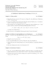
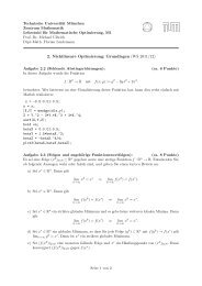
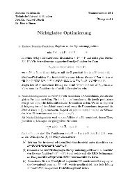
Adjoint Approach to Shape Optimization for Navier Stokes Flow 17(0,0.41)noslip(2.2,0.41)Γ inΓ BΓ out(0,0) noslip(2.2,0)Figure 1. DFG-Benchmark flow around a cylinder; sketch of the geometrywe arrive at an optimization problem with 14 design variables, 12 of which are free(2 design parameters are fixed as we have to ensure that the y-coordinates of thefirst and last B-spline curve points equal 0.2 in order for the curve to be closed).We compute the mean value of the drag on the object boundary Γ B over thetime interval [0, T] by using the formulaJ((ṽ, ˜p), Ω) = 1 ∫ T ∫ ((ṽ t + (ṽ · ∇)ṽ −T˜f))T Φ − ˜p div Φ + ν∇ṽ : ∇Φ dxdt.0 Ω(5.1)Here, Φ is a smooth function such that with a unit vector φ pointing in the meanflow direction holdsΦ| ΓB ≡ φ, Φ| ∂Ω\ΓB ≡ 0 ∀ Ω ∈ O ad .This formula is an alternative formula for the mean value of the drag on Γ B ,c d := 1 ∫ T ∫n · σ(ṽ, ˜p) · φ dS,T 0 Γ Bwith normal vector n and stress tensor σ(ṽ, ˜p) = ν 1 2 (∇ṽ + (∇ṽ)T ) − ˜p I, andcan be obtained through integration by parts. For a detailed derivation, see [12].Integration by parts in the time derivative shows that (5.1) can also be written asJ((ṽ, ˜p), Ω) = 1 ∫ T ∫ (((ṽ · ∇)ṽ −T˜f))T Φ − ˜p div Φ + ν∇ṽ : ∇Φ dxdt0 Ω+ 1 ∫(5.1)(ṽ(x, T) − ṽ 0 (x)) T Φ(x)dx.TΩThus the drag functional (5.1) has the form (3.6). Moreover, using the well knownembedding Y (Ω) ֒→ C(I; L 2 (Ω) d ) × L 2 0 (Ω) it is easy to see that (ṽ, ˜p) ∈ Y (Ω) ↦→J((ṽ, ˜p), Ω) is continuously differentiable if Φ ∈ W 1,∞ (R 2 ) 2 .Computation of the state, adjoint and shape derivative equations is doneusing Dolfin [14], which is part of the FEniCS project [7]. The optimization iscarried out using the interior point solver IPOPT [22], with a BFGS-approximationfor the reduced Hessian.

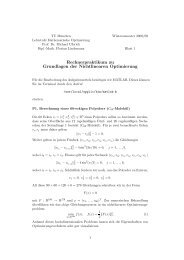
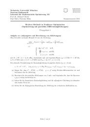
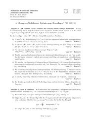
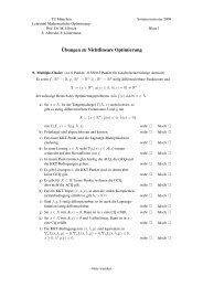
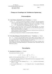
18 C. Brandenburg, F. Lindemann, M. Ulbrich and S. Ulbrich5.2. Choice of shape parameters and shape deformation techniquesOne aspect to consider in the implementation of shape optimization algorithms isthe choice of the shape parameters and the shape deformation technique. Generallyspeaking, shape parameterizations and deformations fall into two classes. Inthe first case, a parameterization directly defines the whole domain, which can beaccomplished by using, e.g., free form deformation. In the second case, the parameterizationdetermines the shape of the surface Γ B of the object B. Examplesfor this kind of parameterizations can be B-splines, NURBS, but also the set ofboundary points Γ B itself, if considered in an appropriate function space. Changesin the shape of the boundary Γ B then have to be transfered to changes of thedomain Ω ref . This can be done in various ways, see, e.g., [2].In our model problem, we have chosen a parameterization of the objectboundary Γ B based on closed cubic B-spline curves [16], where the B-spline controlpoints act as design parameters u. The transformation of boundary displacementsto displacements of the domain is done by solving an elasticity equation, wherewe prescribe the displacement of the object boundary as inhomogeneous Dirichletboundary data [2]. The computational domains Ω k := Ω(τ(u k )) are obtained astransformations of a triangulation of the domain shown in Figure 1. As describedat the end of section 4 we use piecewise linear transformations to ensure a discreteanalogue of assumption (A). Then by an analogue of (3.9) together with thediscrete adjoint equation we obtained conveniently by a continuous adjoint calculusthe exact shape derivative on the discrete level – which we have also checkednumerically.5.3. ResultsThe IPOPT-algorithm needs 15 interior-point iterations for converging to a toleranceof 10 −3 , altogether needing 17 state equation solves and 16 adjoint solves.The drag value in the optimal shape is reduced by nearly one third in comparisonto the initial shape. In the optimal solution, bound constraints for 8 of the designparameters are active, while 6 are inactive. The results of the optimization processare summarized in Table 1.Figure 2 shows the velocity fields for the initial and optimal shape, withsnapshots taken at end time, while Figure 3 shows the computational mesh both forthe initial and the optimal shape. Both meshes are obtained by a transformation ofthe same reference mesh with a circular object, cf. Figure 1, by solving an elasticityequation with fixed displacement of the object boundary.6. Conclusions and outlookIn this paper, we have presented a continuous adjoint approach that can easily betransferred in an exact way to the discrete level, if a Galerkin method in spaceis used. We use a domain representation of the shape gradient, since a boundaryrepresentation requires integration by parts, which is usually not justified on the

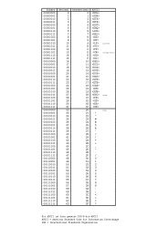
Adjoint Approach to Shape Optimization for Navier Stokes Flow 19iteration objective dual infeasibility linesarch-steps0 1.2157690e-1 1.69e+0 01 1.0209697e-1 1.53e+0 22 9.7036722e-2 3.60e-1 13 8.7039312e-2 6.44e-1 14 8.4563185e-2 5.08e-1 15 8.3512670e-2 1.01e-1 16 8.2813890e-2 1.22e-1 17 8.2516118e-2 8.96e-2 18 8.2069666e-2 1.42e-1 19 8.2062288e-2 1.39e-1 110 8.1995990e-2 1.80e-2 111 8.1994727e-2 6.55e-3 112 8.1995485e-2 2.76e-3 113 8.1995822e-2 2.72e-3 114 8.1995966e-2 1.32e-3 115 8.1995811e-2 2.66e-5 1Table 1. Optimization Resultsdiscrete level. Nevertheless, adjoint based gradient representations can easily bederived from our gradient representation, e.g., for the boundary shape gradient infunction space, but also for shape parameterizations, for example free form deformationor parameterized boundary displacement. The proposed approach allowsthe solution of the state equation and adjoint equation on the physical domain.Therefore existing solvers of the partial differential equation and its adjoint canbe used.We have applied our approach to the instationary incompressible Navier-Stokes equations. In the context of the stabilized cG(1)dG(0) method – but alsofor other Galerkin schemes and other types of partial differential equations – wewere able to derive conveniently the exact discrete shape derivative, since ourcalculus is exact on the discrete level, if some simple rules are followed.The combination with error estimators and multilevel techniques is subject ofcurrent research. Our results indicate that these techniques can reduce the numberof optimization iterations on the fine grids and the necessary degrees of freedomsignificantly. We leave these results to a future paper.References[1] K. K. Choi and N.-H. Kim, Structural Sensitivity Analysis and Optimization 1: LinearSystems, Mechanical Engineering Series, Springer, 2005[2] K. K. Choi and N.-H. Kim, Structural Sensitivity Analysis and Optimization 2: NonlinearSystems and Applications, Mechanical Engineering Series, Springer, 2005

20 C. Brandenburg, F. Lindemann, M. Ulbrich and S. UlbrichFigure 2. Comparison of the velocity fields for the initial andoptimal shape[3] M. C. Delfour and J.-P. Zolésio, Shapes and Geometries; Analysis, Differential Calculus,and Optimization, SIAM series on Advances in Design and Control, 2001[4] K. Eriksson, D. Estep, P. Hansbo, and C. Johnson, Introduction to Adaptive Methodsfor Differential Equations, Acta Numerica, pp 105-158, 1995.[5] K. Eriksson, D. Estep, P. Hansbo, and C. Johnson, Computational Differential Equations,Cambridge University Press, 1996.[6] L. C. Evans Partial Differential Equations, Graduate Studies in Mathematics, AmericanMathematical Society, 1998[7] FEniCS, FEniCS Project, http//www.fenics.org/, 2007[8] P. Guillaume and M. Masmoudi, Computation of high order derivatives in optimalshape design, Numer. Math. 67, pp. 231-250, 1994[9] J. Haslinger and R. A. E. Mäkinen, Introduction to Shape Optimization: Theory,Approximation, and Computation, SIAM series on Advances in Design and Control,2003[10] J. G. Heywood, R. Rannacher and S. Turek, Artificial boundaries and flux and pressureconditions for the incompressible Navier-Stokes equations, Int. J. Numer. MethodsFluids 22, pp. 325–352, 1996.

Adjoint Approach to Shape Optimization for Navier Stokes Flow 21Figure 3. Comparison of the meshes for the initial and optimal shape[11] M. Hinze and K. Kunisch, Second order methods for optimal control of timedependentfluid flow, SIAM J. Control Optim. 40, pp. 925–946, 2001.[12] J. Hoffman and C. Johnson, Adaptive Finite Element Methods for IncompressibleFluid Flow, Error estimation and solution adaptive discretization in CFD: LectureNotes in Computational Science and Engineering, Springer Verlag, 2002.

22 C. Brandenburg, F. Lindemann, M. Ulbrich and S. Ulbrich[13] J. Hoffman and C. Johnson, A New Approach to Computational Turbulence Modeling,Comput. Meth. Appl. Mech. Engrg. 195, pp. 2865–2880, 2006.[14] J. Hoffman, J. Jansson, A. Logg, G. N. Wells et. al., DOLFIN,http//www.fenics.org/dolfin/, 2006[15] B. Mohammadi and O. Pironneau, Applied Shape Optimization for Fluids, OxfordUniversity Press, 2001[16] M. E. Mortensen, Geometric Modeling, Wiley, 1985[17] F. Murat and S. Simon, Etudes de problems d’optimal design, Lectures Notes inComputer Science 41, pp. 54–62, 1976.[18] J. Sokolowski and J.-P. Zolésio, Introduction to Shape Optimization, Series in ComputationalMathematic, Springer, 1992[19] R. Temam, Navier-Stokes Equations: Theory and Numerical Analysis 3rd Edition,Elsevier Science Publishers, 1984.[20] M. Schäfer and S. Turek, Benchmark Computations of Laminar Flow Around aCylinder, Preprints SFB 359, No. 96-03, Universität Heidelberg, 1996[21] M. Ulbrich, Constrained optimal control of Navier-Stokes flow by semismooth Newtonmethods, Systems Control Lett. 48, pp. 297–311, 2003.[22] A. Wächter and L. T. Biegler, On the Implementation of a Primal-Dual InteriorPoint Filter Line Search Algorithm for Large-Scale Nonlinear Programming, Math.Program. 106, pp. 25-57, 2006.[23] W. P. Ziemer, Weakly Differentiable Functions, Graduate Texts in Mathematics,Springer, 1989Christian BrandenburgFachbereich MathematikTechnische Universität DarmstadtSchloßgartenstr. 764289 DarmstadtGermanye-mail: brandenburg@mathematik.tu-darmstadt.deFlorian LindemannLehrstuhl für Mathematische OptimierungZentrum Mathematik, M1TU MünchenBoltzmannstr. 385747 Garching bei Münchene-mail: lindemann@ma.tum.deMichael UlbrichLehrstuhl für Mathematische OptimierungZentrum Mathematik, M1TU MünchenBoltzmannstr. 385747 Garching bei Münchene-mail: mulbrich@ma.tum.de

Adjoint Approach to Shape Optimization for Navier Stokes Flow 23Stefan UlbrichFachbereich MathematikTechnische Universität DarmstadtSchloßgartenstr. 764289 DarmstadtGermanye-mail: ulbrich@mathematik.tu-darmstadt.de