Deciphering Transcriptional Regulation

Deciphering Transcriptional RegulationComputational ApproachesByEivind ValenA dissertation submitted to the University of Copenhagen in partial fulfillment of therequirements for the degree of Ph.D. at the Faculty of Science, University ofCopenhagen.December 2009Supervisors:Assoc. Prof. Albin SandelinProf. Anders KroghAssoc. Prof. Ole WintherD E P A R T M E N T O F B I O L O G YU N I V E R S I T Y O F C O P E N H A G E N

“I may not have gone where I intended to go, but I think I have ended upwhere I needed to be.”-Douglas Adams

AbstractThe myriad of cells in the human body are all made from the same blueprint: the humangenome. At the heart of this diversity lies the concept of gene regulation, the processin which it is decided which genes are used where and when. Genes do not functionas on/off buttons, but more like a volume control spanning the range from completelymuted to cranked up to maximum. The volume, in this case, is the production rate ofproteins. This production is the result of a two step procedure: i) transcription, in whicha small part of DNA from the genome (a gene) is transcribed into an RNA molecule (anmRNA); and ii) translation, in which the mRNA is translated into a protein. This thesisfocus on the first of these steps, transcription, and specifically the initiation of this.Simplified, initiation is preceded by the binding of several proteins, known as transcriptionfactors (TFs), to DNA. This takes place mostly near the start of the gene knownas the promoter. This region contains patterns scattered in the DNA that the TFs can recognizeand bind to. Such binding can prompt the assembly of the pre-initiation complexwhich ultimately leads to transcription of the gene. In order to achieve the regulationnecessary to produce the multitude of tissues we observe, there exists a wide range ofthese TFs having different binding preferences and targeting different genes. By activatingdifferent TFs in a context dependent manner the organism can produce customizedsets of proteins for each cell resulting in different cell types.This thesis presents several methods for analysis and description of promoters. Wefocus particularly the binding sites of TFs and computational methods for locating these.We contribute to the field by compiling a database of binding preferences for TFs whichcan be used for site prediction and provide tools that help investigators use these. Inaddition, a de novo motif discovery tool was developed that locates these patterns inDNA sequences. This compared favorably to many contemporary methods.A novel experimental method, cap-analysis of gene expression (CAGE), was recentlypublished providing an unbiased overview of the transcription start site (TSS) usage ina tissue. We have paired this method with high-throughput sequencing technology toproduce a library of unprecedented depth (DeepCAGE) for the mouse hippocampus. Weinvestigated this in detail and focused particularly on what characterizes a hippocampuspromoter. Pairing CAGE with TF binding site prediction we identified a likely keyregulator of hippocampus.Finally, we developed a method for CAGE exploration. While the DeepCAGE librarycharacterized a full 1.4 million transcription initiation events it did not capturethe complete TSS-ome of hippocampus. We fitted two statistical models to the CAGEdata and extrapolated how deep sequencing needs to be to capture most of the events.We concluded that while most genes are discovered, tag clusters and TSSs are not fullyexplored.v

IntroductionEvery organism on this planet consists of one or more small basic functional units.These building blocks of life are known as cells and come in two basic forms: prokaryoticand eukaryotic. The major difference between these is that the eukaryotic is largerand have several specialized sub-compartments called organelles. The prokaryotic cellsare the choice of many unicellular organisms including two of the major branches of life:bacteria and archaea. Most multicellular organisms have more demanding organizationand the vast majority of these are therefore eukaryotic.Residing within these cells lies our basic hereditary material. As is common knowledgenow this consists of deoxyribonucleic acid (DNA). DNA is a long molecule builtfrom small basic building blocks: the nucleotides. These come in four different flavors:adenine, cytosine, guanine and thymine that fits together in pairs. Adenine can bond (orbasepair) with thymine and cytosine can basepair with guanine. Assembled sequentiallythese form a long strand of pairs that is twisted around itself forming the famous doublehelix. Since the DNA in its native form is of substantial length it is usually packedinto a compact structure known as chromatin. Besides the DNA, chromatin consists ofa set of basic proteins called histones that the DNA is wound around which can attaincondensed conformations.A complete collection of DNA is known as a genome and for many organisms is oftendivided into smaller chunks known as chromosomes. In the eukaryotic cell these residemainly in a large organelle: the nucleus, but a small part is present in many copies witheach one placed in a comparably tiny organelle: the mitochondrion.Spread across the DNA of each chromosome lies segments known as genes. Whilethe exact definition of a gene is debatable and somewhat complex, a simplified definitionwould be: a segment of DNA forming a blueprint for a protein. This happens intwo steps. The first, transcription, is facilitated by a protein using the gene DNA as atemplate for making a complementary ribonucleic acid (RNA) strand. The RNA is constructedby basepairing RNA to the DNA and then releasing the RNA product. This ispossible because RNA is very similar to DNA just having a different backbone linkingthe nucleotides into strands. It also has a replacement for the nucleotide thymine knownas uracil which can also basepair to adenine. Due to the rules of basepairing the newRNA molecule will now be the exact complement of the DNA template and is known asa transcript or messenger RNA (mRNA) 1 . Transcription starts at the transcription startsite (TSS) residing at the very beginning of the gene in an area known as the promoterregion and proceeds to the transcription termination site.After a mRNA has been produced and undergone some processing it is exportedout of the nucleus and into the cytosol which is the large space outside the organelles.1 At this point technically a pre-mRNA1

2Here the second of the two steps, translation, take place. This is the process where aprotein is produced based on the mRNA transcript. The main actor in this process is thelarge protein complex (a collection of many proteins and other molecules) known as theribosome. Proteins are the basic building blocks of the cell and, similar to DNA, theirprimary structure is a long chain of smaller components. In this case they are calledamino acids and there exists about 20 of them. Since the mRNA transcript consists ofjust 4 elements and a protein has 20 elements a certain language or code is needed totranslate between the two “alphabets”. This translation is known as the genetic codeand is with some exceptions universal to all life. The basic idea is that 3 nucleotides(a codon) uniquely identifies one amino acid 2 . The translation is performed by smallcloverleaf shaped molecules known as transfer RNAs (tRNAs) of which there are manytypes. Each of them can basepair with a codon at one end, using the region knownas the anticodon (consisting of the complementary bases of the codon) and can have acertain amino acid corresponding to the anticodon attached to the other end. Using thissystem, the tRNAs can basepair with the next three nucleotides on the mRNA bringingwith it the correct amino acid. This is then attached to the previous amino acids forminga chain. The ribosome makes sure that the mRNA is processed sequentially so that theamino acids are assembled in the correct order.At the turn of the millennium a gargantuan task was nearing completion. Large headlinesappeared in the papers that the human genome was finally sequenced promisingto bring a cornucopia of benefits to medicine and basic understanding. Sequencing ofDNA is the process of figuring out the order the 4 types of basepairs are arranged in on aDNA molecule. In the case of the human genome project the DNA was the 24 differentchromosomes and 3.3 billion basepairs that the human genome consists of. It was theculmination of ten years of hard labor and 3 billion dollar in expenses, but sequencingtechnology has progressed a lot since then. For comparison the company Illumina recentlyannounced that it could do full genome sequencing for $48,000 and it is expectedthat the $1000 genome will soon be within reach.With the sequencing of an ever increasing number of genomes, one of the majorchallenges ahead is to understand how these blueprints result in the diversity of cellsand behavior we see in every organism. In humans, liver cells are radically differentfrom those of the cerebellum yet they both share the same genome. The difference liesin the interpretation of this recipe and deciding which genes and proteins are turned onand off during their life-time.At the heart of the diversity lies the concept of gene regulation. This is a multifaceted,messy and hugely interconnected machinery featuring a plethora of cooperative andantagonistic agents that work on various steps and levels in the life cycle of the cell.Genes do not simply have on/off buttons, but function more akin to a volume control.They can be everything from more or less mute to turned up to maximum, cranking outRNAs at an alarming pace. While there are no actual buttons, the machinery takes cuesfrom signals superimposed or encoded in the vicinity of the genes, binding agents thatinhibit or stimulate the transcriptional expression.Isolated, the in silico representation of the genome is only a long string of letters2 Since 4 3 = 64 multiple triplets code for the same amino acid

(A,C,G and T representing each of the four nucleotides). For most organisms thesestrings are of a magnitude that makes human curation and interpretation impractical,hence the introduction of bioinformatics or computational biology. Building upon along tradition in computer science and machine learning, it has rapidly gained popularitydue to its necessity in the age of high-throughput experiments. Through the diligentapplication of both experimental and computational methods, patterns have started toemerge in the genome. These can make sense of how the cell is able to keep track ofwhat is supposed to be expressed, how much and where.The steps of transcription and translation provides at least two levels where regulationof this expression can act. This is naturally a simplistic view, almost deceivingly so, aswe are continually observing RNAs that are not translated into proteins and are functionalin and of themselves. These non-coding RNAs (ncRNA) are abundant and manyof them seem to affect the production and life-cycle of other RNA molecules [1–5].3

4Transcription Initiation by RNA PolII and the CorePromoterThe general principles underlying the transcriptional machinery is the same for prokaryotesand eukaryotes, but is in the latter case much more complex. In bacteria and archaeatranscription is carried out by a single enzyme: RNA polymerase (RNA Pol) while ineukaryotes there are three (I-III) used depending on the final product where RNA PolIIis the one responsible for protein coding genes.Transcription facilitated by RNA PolII can be roughly divided into three phases: i)initiation, where the factors assemble on the promoter and transcription starts; ii) elongation,where transcription moves out of the promoter and through the gene; and iii) termination,when RNA PolII reaches the end of the transcript and stops. Additional stepsoften included are “pre-initiation” being the formation of the so-called pre-initiationcomplex (PIC) and “promoter clearance” between initiation and elongation which, dueto its complexity, merits its own stage. Several studies have targeted the complex behaviorof the polymerase during this phase [6, 7]. This thesis however, will mainly focuson some of the more traditionally recognized steps of regulation: the involvement oftranscription factors (TF) in transcription initiation and the concept of promoters particularlyin light of new experimental techniques.The DNA-dependent RNA PolII has the ability to unwind and rewind DNA as well assynthesize RNA [8], but it requires help in the recognition of promoter sequences shownby in vitro attempts to reproduce mRNA transcription [9,10]. RNA PolII therefore formsa larger system, the PIC, that assembles on the DNA. It comprises six proteins: RNAPolII and the five basal/general transcription factors: TFIIB, TFIID, TFIIE, TFIIF andTFIIH. In total over 30 polypeptides, but the exact subunits can vary according to thetissue and promoter type [11]. Various openings facilitate nucleotide access and exitfor the RNA [12, 13]. Close to the exit lies the carboxyl terminal domain (CTD) of thelargest subunit of RNA PolII. This contains a repeat sequence that is bound by severalproteins involved in processing the RNA as it leaves the transcriptional complex.Early promoter studies were mostly performed on highly expressed promoters, oftentissue specific and with the property that they could easily be induced. Most of thesecontained an AT-region approximately 30bp upstream of the TSS termed the TATA-boxafter its consensus sequence. This element was discovered in 1979 by comparing 5’flanking sequences of genes from Drosophilia [14]. It was also revealed that the TATAbindingprotein (TBP), a subunit of TFIID, was an essential part of the initiation complexthat bound to this element. Thus the picture emerged that a promoter consisted ofa TATA element surrounded by other more variable elements that produced differentialexpression.The promoter core elements were initially believed to be invariant, but further studiesrevealed that not all promoters contained a TATA-box. In addition they could alsocontain other recurring patterns that were shown to be functional. Among these werethe initiator element (INR), TFIIB recognition element (BRE) and the downstream promoterelement (DPE) [15], where BRE is recognized by TFIIB and INR and DPE arerecognized by TBP associated factors (TAFs). A given promoter could contain none,

5one or more of these, but rarely many at the same time. Recently, other signals not partof the DNA, but instead modification made to the DNA packaging material: histoneshave been shown to facilitate binding. In particular a trimethylation of the amino acidlysine on the fourth residue of the histone 3 (H3K4) has been shown to promote bindingby TFIID [16].In addition to various novel core elements other findings also emerged to challengethe old dogma. Studies showed examples of promoters that had multiple initiation siteschallenging the assumed specificity of TSS usage. Despite this, the TATA-box promoterwith a single initiation site prevailed as the image of a typical promoter and is still theone most often presented in textbooks.Transcription Factors and their Binding SitesWhile the core initiation complex is required for transcription, it is certainly not the onlyagent involved. To achieve differential expression across genes, evolution has producedan abundance of trans-acting TFs that act on various cis-regulatory elements present inthe vicinity of their target genes. By binding in proximity to their targets these act byrepressing or activating their targets through chromatin modifications, recruitment ofco-factors, or direct interaction and summoning of the PIC.Unlike the TATA-box which is a general motif present in a multitude of genes thesecis-elements can be limited to small groups of, and in some cases only, genes involvedin very specific, rarely used pathways. Consequently, the TF or TFs 3 that targets thiselement may only activate or repress a small collection of genes. Such targeted regulationis not uncommon and by having different cis-elements at different promoters anddifferent transcription factors active in different contexts the cell can tightly regulatewhich genes are expressed at any given time during its lifetime.To target a particular binding site it is necessary that TFs have certain preferences forthe DNA that it binds to, binding strongly to some sequences and weakly to other. Theactual binding site we will refer to as a transcription factor binding site (TFBS) whilethe model that attempts to represent and summarize the binding preferences of a TF willbe referred to as a motif.TFBSs can take many forms and it was shown early on that unlike restriction enzymeswhich have very specific targets, TFBSs can display considerable variance. An exampleof this can be seen in the λ operators which contain 12 half-sites where only two out ofeight positions are completely conserved [17]. The reason for this lack of specificity isassumed to stem from the advantages this provides in regulating expression. As differentinstances of the motifs provide different binding efficacy, the promoter can be finetunedto provide a certain transcriptional output for that gene [18]. Since TFs also targetmultiple genes, a single factor can give rise to a wide range of output for its target genesusing this system.TFBSs are often fairly small, on the order of 6-20 bases. The longer ones are rarelyconserved across the whole length, but often consists of two half-sites separated by a3 Different TFs may target the same cis-regulatory elements

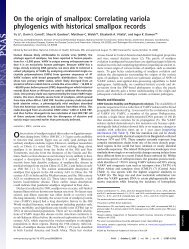
6stretch of non-informative bases. A few are palindromic and many resemble each otherand are closely targeted by classes of factors with similar binding profiles.The quest to understand sequence specific binding started with the lac operon andthe discovery that the regulation of expression was connected to a protein factor [18].Concurrently with the experimental work, theoretical analyzes were being performed tounderstand the amount of information required for the functioning of regulatory systems[19, 20]. TFs are now understood to be highly dynamic, diffusing rapidly through thenucleus, directed to their sites partly by their transient binding to chromatin [21]. Theymay associate with DNA all over the genome, but having affinity for certain sequencesensures that the TFs spend more time at these positions thus increasing or preventingthe chance of PIC assembly.Unfortunately, the detection of these binding sites is complicated by their weak spatialrestrictions. While most binding sites are assumed to bind in the vicinity of theTSS in the so-called proximal promoter region [22], many binding sites shown to befunctional are clearly nowhere near this. Instead, these can reside in distal sites oftentens of thousands of Kbp away (Fig. 1) and are then usually referred to as enhancers orsilencers.Figure 1: Transcription factor binding sites (TFBS) can reside in the proximal promoterregion or in more distal sites. Often sites cluster together into so-called cis-regulatorymodules (CRM). Figure from [23].

8Figure 2: The type 0 cap structure. Figure from Wikipedia licensed under CreativeCommons.After sequencing, the 20bp long sequences called ’tags’ can be mapped to the genomeusing short read mappers such as bowtie [30] or bwa [31]. This effectively gives a genomicview over the transcription start site usage of the cell only limited by the sequencingdepth. Also, since transcripts are sampled roughly proportionally to their abundancein the cell, CAGE correlates with the relative expression of each start site.An initial surprise emerging from the first runs was that it appeared that most promotersdid not conform to the TATA-box archetype. In fact the majority of promotersappeared to lack this particular element and could rather be characterized by their associationwith CpG rich regions termed CpG islands. Additionally, and perhaps the mostsurprising, a single initiation site for each gene seemed to be the exception rather thanthe rule. Instead most genes featured a distribution of TSSs where some were favoredabove others [33–35]. The initial reaction to this was of one disbelief and suspicion ofexperimental noise, but it was quickly realized that noise was not an adequate explanationfor the observed data. In particular the following reasons were considered [36]:• The classical single TSS, TATA-box-containing promoters were still observed albeitas a minority in the total population of promoters. These were positionallyhighly constrained across all tissues were the gene was expressed.• In the broader promoters the relative distribution of tags were often preservedacross many tissues. This is not compatible with random experimental noise. Thiswas also observed across the species barrier as one discovered similar promoterdistributions in human and mouse.

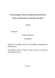
Figure 3: The CAGE protocol in 9 easy steps. Figure from [32].9

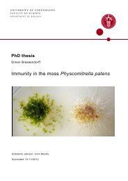
10After concluding that most genes were not too particular about their TSSs it quicklybecame apparent that it was beneficial to group these TSS into units reminiscent of theclassical promoter. This was motivated by the fact that proximity made it likely thatthey shared regulatory input or were subject to the same constraints on nucleosomeoccupancy. To begin with, one grouped all tags that mapped to the same 5’ positioninto a CAGE-tag start site (CTSS) and used these to further cluster (based on overlapof tags) into larger units called tag clusters (TC) [34]. The TC including some of thesurrounding sequence corresponds roughly to what in classical terms was known as thecore promoter. As the overlapping of tags is a somewhat arbitrary criteria for clusteringlacking a clear biological motivation more sophisticated clustering methods takingco-expression and strength (number of tags) into account were later devised [37, 38] togroup TSS that have a high probability of being subject to the same regulatory machinery.Given that one observed such different promoters as the TATA-box, single peak typeand the broader, usually TATA-less and often CpG-associated types it was natural toclassify the TCs into distinct categories. The first attempts at this divided the promotersinto four categories (Fig. 4) [34], but this is often simplified into just a single peak (SP)category with 75% of the tags within 4nt of each other and a broad (BR) category whichis a catch-all term for everything else.Another surprise CAGE uncovered was the extensive use of alternative promoters.Some TCs targeting the same gene were clearly too far apart to be considered the samepromoter. In fact the initial study revealed that 50% of known genes had two or morealternative promoters which is undoubtedly an underestimate. They are often clearlyindependently regulated and in those cases where you have multiple promoters each ofthem often show clear tissue preferences. Such a system makes it possible for a geneto have two different inputs which can help to organize differential regulation. Furthermore,it can also give rise to several different mRNAs and as such be a complement toalternative splicing.

Figure 4: The four types of promoters classified by Carninci et al. [34]. Figure fromthe same paper.11

12Computational Sequence AnalysisIdentifying cis-regulatory elements and their shared motifs by experimental means canbe an arduous task as experimental procedures have been either time-consuming (genereporter/deletion assays) or lacking in the base level resolution that would be desirable(CHiP-chip [39]/CHiP-seq [40]). As a consequence much effort has been invested inproducing computational methods as an alternative to experiments or as a complementto assays with lower resolution. Predictions from high quality methods can also be usedto form hypotheses which could later be subjected to the more expensive, tedious andtime consuming process of experimental verification. Furthermore, good models couldshed light on the intrinsic features of the binding process and insight gleaned from theconstruction of these may increase our general knowledge of the nature of TF bindingwhich could be exploited when new genomes are sequenced.When discussing computational searches for motifs it is helpful to distinguish twodifferent, but similar problems:• In the first we know which motif we are searching for and are merely interestedin its presence/absence or its position. I will refer to this as “motif finding” 4 .• In the second we suspect that some sites are present, but we do not know what themotif is nor the sites’ position. I will refer to this as “motif discovery”.Note that these are not universal terms. They vary and are sometimes used interchangeablyin the literature.In both instances, it is common to start with a set of genes of interest derived fromexperiments or experience. Typically, one selects genes that are co-expressed and byextensions suspected to be under the control of the same regulatory machinery. Sharedtranscription factors often implies common motifs so this increases the likelihood offinding similar binding sites. Both “finding” and “discovery” are basically a matterof differentiating between signal and noise. The signals are the binding sites and everythingthat is usable in their detection and the noise is everything else. Besides thebinding sites themselves there can be several other sources of information. Among themore popular is evolutionary conservation exploited in phylogenetic footprinting [41]and expression data which can be used to infer in which sequences the binding sites aremost likely to be found [42].Broadening our scope from a single factor, there are also many signals discerniblein the interaction between factors. TFs often operate in larger groups known as cisregulatorymodules and we can infer information by looking at how the individual TFinteracts at single promoters or across the genome.De novo motif discovery is often aimed at either single motifs or the interaction ofa few motifs since optimization of objective functions modelling larger contexts canbe computationally hard. Interactions should in this case not be confused with simplysearching for multiple motifs in a set of sequences which many motif discoverers do,but rather explicit modelling of co-occurrence. Motif finders on the other hand, starting4 Other terms sometimes used in the literature are “motif scanning” and “motif searching”

15Table 2: Various matrices for the transcription factor ELK1 made from the above alignment(Fig. 5) and 18 other sites.(a) Count matrix1 2 3 4 5 6 7 8 9 10A 7 10 9 5 2 0 1 27 21 13C 7 6 4 19 24 0 0 0 5 0G 10 6 10 1 1 24 27 1 0 14T 4 6 5 3 1 4 0 0 2 1(b) Probability matrix1 2 3 4 5 6 7 8 9 10A 0.25 0.36 0.32 0.18 0.07 0.00 0.04 0.96 0.75 0.46C 0.25 0.21 0.14 0.68 0.86 0.00 0.00 0.00 0.18 0.00G 0.36 0.21 0.36 0.04 0.04 0.86 0.96 0.04 0.00 0.50T 0.14 0.21 0.18 0.11 0.04 0.14 0.00 0.00 0.07 0.04(c) PSSM with a pseudocount of 0.11 2 3 4 5 6 7 8 9 10A 0.00 0.51 0.36 -0.48 -1.76 -6.15 -2.69 1.93 1.57 0.88C 0.00 -0.22 -0.79 1.43 1.76 -6.15 -6.15 -6.15 -0.48 -6.15G 0.51 -0.22 0.51 -2.69 -2.69 1.76 1.93 -2.69 -6.15 0.99T -0.79 -0.22 -0.48 -1.20 -2.69 -0.79 -6.15 -6.15 -1.76 -2.69could be made that one should only consider places where it is not impossible for thefactor to bind.All of the above mentioned models have in common that they consider each positionin the motif to be independent of the others. While this is a nice property when doingcalculations it is not simply something we can assume is true. Fortunately for us,while interdependencies do exists [45] in most cases assuming independence is a goodapproximation [46].Despite this observation some attempts have experimented with higher-order models.This includes higher-order matrices and Markov models. A major roadblock for this haslong been the lack of data necessary to fit the increased number of parameters, but withthe introduction of high-throughput methods like CHiP-seq this should no longer be ahindrance.Motif findingMotif finding is the scenario where you have both motif model(s) and a set of sequencesthat you want to study. The models are usually compiled from experimental data (e.g.SELEX [47]) or a combination of this and computational methods (CHiP-seq [40] +motif discovery) which we will discuss in the next section. Recently k-mer arrays havebeen introduced [48] which have the potential to elucidate the binding preferences of

16Figure 6: Logo of the binding preferences for the ELK1 transcription factor. Madefrom an alignment of 28 binding sites.TFs in a comprehensive fashion. Several databases contain compilation of these motifsmostly in the form of WMs. JASPAR ( [49, 50], paper II), TRANSFAC [51] andUniPROBE [52] are among the most well known.When using a consensus sequence, motif finding is fairly straightforward. It is simplya matter of iteratively scanning through the sequences and seeing if any sites are presentor not. However, knowing that sites are often variable one would normally allow somedeviance from the consensus in the form of mismatches. This should be weighed upagainst the increasing number of false positives that we will identify if allowing toodivergent sites. Using TATAAT as an example, given a random uniform sequence wecan expect to see this every 4 6 = 4096 nucleotide. Allowing one mismatch this numberis suddenly 46 = 227 which given a typical range (e.g. -300 - +100 around the TSS)3∗6for searching a promoter would be expected to include at least one site by random.For weight matrices the problem is somewhat more complicated. To assess whethera binding site for a probability matrix w of length |w| is present at a certain location iin sequence X one multiplies the probabilities from the weight matrix corresponding tothe letter present in the sequences:|w|∏P (X i |w) = w Xi+j ,j (3)This gives the probability of the sequence given the weight matrix model. However,since long products of probabilities approach 0 quite rapidly this has the unfortunateconsequence that computers (being poor at representing real numbers) experience problemsaccurately keeping track of the product 5 . Therefore, it is customary to use logtransformed values and summing these instead:j=1|w|∑log 2 P (X i |w) = log 2 w Xi+j ,j (4)j=15 This phenomenon is in computer science known as underflow.

17The base two is a traditional computer science choice giving results in the unit “bits”.As before we would like to also consider the background of the genome to give us someindication of how surprising a certain result is. We can transform the probability matrixw by dividing with the background probabilities q and taking the logarithm (usually base2) giving us what is known as a position specific scoring matrix (PSSM) (Fig. 2(c)):P SSM b,i = log 2w b,iq b(5)This can be used to score sequences by summing over the cells corresponding to thesequence, where any score over 0 is more likely to be a product of the motif model ratherthan the background. It is also customary to add a small pseudocount to each cell in thematrix before transforming. The justification for this is that the data the matrix is builtfrom is rarely complete and there is a big difference in having minuscule probabilityand a probability of 0. In addition log is not defined for 0 making the transformationproblematic.While a score larger than 0 indicates a higher probability of being generated by themotif rather than the background one rarely considers hits close to 0 as significant.Instead, a threshold is often used considering everything above as a real binding site.This can be calculated in various ways:• Based on prior assumptions of how often the motif should occur [53].• Based on how often it is deemed acceptable to occur in what is assumed to benon-regulatory sequences [54].• Based on the scoring range possible using the PSSM. For instance 80% of themaximum achievable score.No matter how one calculates the threshold, it is an ad hoc way of separating thewheat from the chaff based on the assumption that most PSSM-predicted binding sitesare not involved in transcription factor binding. The assertion that most of these sitesare not functional is known as the “futility theorem” [23]. Seen in the light of recentdiscoveries [21] it is likely that many of these are bound in vivo as well as in vitro, butthat other conditions are not fulfilled for PIC assembly (e.g. other factors or histonemodifications). Consequently, these events rarely lead to initiation.Motif discoveryIn motif discovery we also start out with a set of sequences that we are interested in, butunlike motif finding we do not know what pattern we are looking for. This is usuallyperformed after first attempting motif finding since it is advantageous to exclude allknown factors before attempting to discover new ones. The problem is analogous tothe problem of finding optimal local multiple alignments and therefore, by reduction,belongs in the infamous class of intractable problems known as NP-complete [55].Motif discovery is considered to be one of the classical problems in bioinformaticsdating back at least 27 years [43]. As a consequence there are by now literally hundreds

18of methods developed all varying in their choice of model or optimization. However, allof them rely on some common assumptions.The primary reason computational prediction is at all possible is that the motif youare searching for is in some way over-represented compared to what is expected. Thiscan be as simple as that a consensus sequence (e.g. TATAAT) occurs in every sequence,to the more realistic test that the number of times a PSSM scores above some specificthreshold is greater than would be expected if the sequences were generated by a higherorderbackground model.One can distinguish two approaches to the background model. In most cases thisis modelled by a multinomial or higher order Markov chain that gives frequencies forthe nucleotides, but lately more methods using a discriminative approach have beenattempted [56, 57]. Discriminative in this context means that you have an additional setof sequences (a negative set) that are used to contrast with the set you suspect contain themotifs (the positive set). The advantage to this is that given a representative backgroundit can perform better than any model approximation of this.Additional constraints could also be added to get a more nuanced picture of the expectedfrequencies. For instance one could look at the position based over-representationnoting that while TATAAT may not in itself be over-represented it could be the case thatit is over-represented in the region -30 to -25 relative to the TSS. Sadly, such constraintsare rarely as specific as in the case of the TATA-box. While most sites are in the vicinityof the TSS there is no guarantee they will have strict spatial constraints.In addition to a motif model most methods feature an objective function describingwhat is a good configuration and how to interpret over-representation. This shouldcapture whether whether motifs have to be present in each sequence (one occurrenceper sequence (OOPS)), whether sequences without motifs are tolerated (zero or OOPS(ZOOPS)) or whether multiple motifs per sequence are allowed. It is also importantin defining the nature of the motifs: are you trying to maximize information content,number of motifs, discriminative potential or a combination of these?Finally, an algorithm for optimizing this function is needed. The choice of this islargely dependent on the motif model and objective function. Most methods fall intoone of two categories: enumerative or statistical optimization methods, the latter canbe further subdivided into deterministic and stochastic methods. Enumerative strategiesproceed by in some way going through (“enumerating”) all possible motifs of a certaintype. This is often used in conjunction with a sequence-based motif model. A goodexample is the Weeder algorithm [58] which explores sequences of length N with upto m mismatches. Statistical optimization on the other hand attempts to optimize anobjective function through general or ad hoc optimization strategies. The Gibbs sampler[59] is one example using the Gibbs sampling method to optimize a weight matrix.Some other algorithms that have been attempted are expectation maximization [60],perceptron learning [57] and independent component analysis [61].The accuracy of motif discovery tools has been fairly poor throughout the life timeof the field. The main problem stems from the small size of motifs compared to thesurrounding sequences. The positions with high information content are usually fairlyshort (6-8 bases) and can be hard to detect in the sea of noise surrounding it. This

phenomenon of a too low signal to noise ratio is often known as“pattern drowning”and unfortunately affects many analyzes. To make things more difficult there are nohard rules for where motifs can be located only rough guidelines or conventions thathave emerged. Typically, one ignores possible enhancers and silencers unless one hasspecific knowledge of their location. Instead it is common to search either the -300 to+100 region around the TSS or the -1000 to +200 region. The former choice is motivatedby the fact that when plotting the mean evolutionary conservation of all promoters ittends to drop dramatically around the 300 mark. The latter choice is more motivated bythe limits of pattern discovery tools. Both regions are asymmetric for the simple reasonthat searching far downstream quickly puts you in the middle of the coding region whichhas its own strongly biased sequences. However, recent investigations have shown thatmany sites are distributed symmetrically around the TSS [22]. Given that this is truethis would indicate that many older results using these regions are possibly biased.19

Present Investigation“It’s sometimes called the final frontier. (Except that of course you can’thave a *final* frontier, because there’d be nothing for it to be a frontier*to*, but as frontiers go, it’s pretty penultimate...)”-Terry PratchettThe goal of promoter analysis is to elucidate the biological functions that produce theobserved patterns. While the complete understanding of this lies beyond the ambitionof this thesis, several steps have been made towards this goal. Some of the sub-goalsinclude:• Improvement of the historically poor performance of motif discovery tools.• Extending the existing collections of motifs for transcription factors.• Integration of these collections with tools to aid in the search for regulatory sites.• Identification of key regulators in tissues by combining experimental data andcomputational predictions.• Estimating the complexity of transcription initiation for tissues.• Developing methods to deal with high-throughput tag data.The four papers included in this thesis each addresses one or several of these points.Paper I is a contribution to the motif discovery field featuring a novel discriminatoryapproach out-competing many contemporary methods.Paper II extends the largest open-access collection of motifs and introduces severalextensions and tools to help in this process.Paper III presents the largest mapping of promoters in primary tissue to date. It uses anovel experimental technique paired with motif finding to identify one of the keyregulators of this tissue.Paper IV is the first attempt to estimate the size of the promoterome and TSS-omebased on CAGE data.21

22Paper I: Discovery of Regulatory Elements isImproved by a Discriminatory ApproachWhile published towards the end of my PhD, this paper marks the beginning of myventure into bioinformatics and addresses one of the fields’ classical problems: de novopattern finding or “motif discovery”.In particular, it is aimed at pattern finding in relation to transcription initiation. Asdiscussed previously, transcription initiation is subject to control and regulation by severalproteins termed transcription factors that can bind in the vicinity of the TSS. Bybioinformatical standards this is an old field and by now there are literally hundreds ofmethods developed to attack this problem. Despite this, few are tested as extensively aswe do in this article. This includes comparison to some of the more famous tools likeMEME [60] and Weeder [58] where we compare favorably.Using the classification from the introduction, Motif Annealer (MoAn) is a discriminativestatistical optimization method. The initial aim was to model cis-regulatory modules,but the nature of our model made the search space quite large making interactionshard to optimize. However, we realized that our objective function showed high correlationwith the correct solution on simulated data. This paired with a large negative setresulted in good performance on single motifs. The focus therefore shifted to whetherwe were able to out-compete contemporary methods at this task. Our method still hasthe capacity to model co-occurrence, but for this to be practical the optimization needsto be improved.Comparing our method against the aforementioned tools as well as DEME [56] andNestedMICA [61] shows that our method is better at discriminating between the heterogeneousbackground of the mammalian promoter and transcription factor bindingsites. This was concluded based on both synthetic sets (in line with the recommendationsof a recent large scale evaluation of methods [62]) and on real data fetched fromthe PAZAR database [63]. We experience somewhat better results on the synthetic setswhich we hypothesize may be due to the negative set being more representative of thisbackground.We also show that our method does not rely on the common pre-processing step ofrepeat masking [64]. This is a particularly good feature as some repeats have beenshown to be functional [65, 66] with respect to transcription initiation. Indiscriminateuse of masking, a step required by many methods, may therefore remove real signals.Our method gains its power from two components: i) the large negative set and ii)the objective function. The complexity of scanning naively with a PSSM is linear withrespect to the sequences (each positions is checked once) which would be intractableif the sequence set is sufficiently large. Instead we have implemented a data structurecalled an enhanced suffix array [67–69] which is a more efficient representation of asuffix tree [70]. This, combined with a threshold for PSSM searching, enables us tosearch all the sequences in an efficient manner.As our objective function we use a conditional maximum likelihood for estimatingthe PSSM that best discriminates between the positive and the negative set. We let thematrix vary with counts independent of the sequences and therefore cannot necessarily

e derived from the sequences. The likelihood is formulated as the product over thesequences of the probability of the sequence label (positive/negative) given the sequenceand the WMs.Optimization is performed with a general optimization technique known as simulatedannealing [71]. In short it performs random steps through the search space and thenaccepts or rejects these based on the difference in log-likelihood between the currentand the proposed state. Acceptance is also influenced by a temperature parameter thatgradually shrinks the space of valid moves, accepting fewer and fewer bad ones. Theidea is that after exploring the search space the method gradually converges towards theglobal maxima before finally getting trapped there by the low temperature. At the timeof writing the optimization is the weakest part of this method.23

24Paper II: JASPAR, the open access database oftranscription factor-binding profiles: new contentand tools in the 2008 updateThe JASPAR database was motivated by the lack of an open source, free collection ofbinding motifs for transcription factors. Unlike its commercial competitor TRANSFAC[51], JASPAR focuses on quality before quantity. This is accomplished by using humancurators who ensure that every matrix lives up to experimental standards and that everyfactor is represented by the best available matrix. The original database is highly citedand forms the backbone of many motif-finding applications.This paper describes its third major release and is the culmination of a collaborationbetween the Computational Biology Unit in Bergen and The Bioinformatics Centre. Ithas three main authors focusing on different aspects. Jan Christian Bryne developed aweb service Java library for interaction with JASPAR, Man-Hung Eric Tang focused ondata curation and I developed and extended the functionality of the database throughintegration with tools for dynamic clustering and random profile generation.The release features an extended core database with motifs that passed our qualitystandards as well as three new sub-databases:POLII Core promoter motifs (e.g INR and BRE) [35, 72]CNE Conserved non-coding elements from Xie et al. [73]. Many acting through longrangeeffects as enhancers.SPLICE Splice sites as matching donor acceptor pairs [74]In addition we provided several additional summary statistics showing among otherthings the number of spurious hits you would expect to see in random sets of promoters.We also developed a WS-I compliant Web Service interface. This is coded in Javaand is an API to simplify external utilization of the database. In particular to make iteasier to use JASPAR in workflow managers like Triana [75] or Taverna [76].Another important addition was the functionality to create custom familial bindingprofiles (FBP). Many TFs target similar motifs and by clustering them to a FBP you getmodels describing a set of matrices. This functionality is provided by the underlyingSTAMP [77, 78] tool. This also provides functionality to align matrices to the wholeJASPAR database, searching for the best match. The latter is particularly useful if amotif discovery tool has found a motif you suspect is already known.This release also provides a way of generating ’random’ matrices. This can be usefulin many assessments for instance a scenario where you want to judge the significanceof finding a certain number of sites matching a matrix. It is desirable that the matrices,though random, still share common properties with real binding sites. We thereforeprovide two methods to generate these:• In the first we simply shuffle the columns within a matrix thus generating a newmatrix with the same information content as the first.

25• In the second method we sample random columns using a statistical model. Aposterior distribution consisting of a multinomial using counts from real matricesand a Dirichlet mixture prior trained on the observed nucleotides in the JASPARdatabaseBoth methods assume independence of columns.Since its inception the JASPAR database has become a mainstay of the motif-findingcommunity and is used extensively in our work including paper III and [79–81].

26Paper III: Genome-wide detection and analysis ofhippocampus core promoters using DeepCAGEThis work represents the first instance of the DeepCAGE protocol. DeepCAGE isthe merging of the Cap Analysis of Gene Expression (CAGE) protocol with highthroughputsequencing. In this case the 454 Life Sciences (Roche) GS20 sequencerprovided 2 million randomly primed tags from TSSs used in the mouse hippocampus.At the time of publication this was the most comprehensive landscape of PolII TSSscompiled for any tissue. Of the 2 million, we could unambiguously map 1.4 million tothe mouse genome.This is a technology-driven paper that explores what information one can get by sequencingto this depth. To this end, we compared our data with 7 other tissues: cerebellum,embryo, liver, lung, macrophages, somatosensory cortex and visual cortex compiledfrom a total of 39 libraries.We first clustered all tags based on proximity which resulted in 18,948 TCs. Since thelibraries spanned a wide range of sizes it was necessary to normalize the counts in eachtissue to tags per million (TPMs) to have a basis for comparison. It should be noted thatsince we do not know the actual population size of the transcripts in the cells we canonly compare relative preference within a cell. This is distinct from actual transcriptionstrength, measured in initiation events per time unit. We discuss this further in [82].After normalization we performed hierarchical clustering on the TCs versus the TPMsfrom each tissue for each of these. This showed, as expected, that the brain tissuesare more highly correlated to each other than the rest of the tissues and, in particular,somatosensory and visual cortex are similar in terms of transcription initiation.Seeking to identify the unique features of hippocampus, we sought to identify promotersthat were primarily used in this tissue. Historically one has referred to tissuespecificity, but with the advent of CAGE this term has lost much of its meaning since:• Few TCs have tags exclusively from one tissue.• Compared to all cell types and tissues, we have sequenced relatively few.• Tissues can not be sequenced to infinite depth and in most cases we are far fromdetecting everything (as discussed in paper IV).To address this, we derived the concept of a preferentially expressed promoter (PEP).The PEP definition is not particularly robust to generalization, but focuses on creating asubset that is strongly expressed and over-represented in one tissue for further analysis.In total we ended up with 6536 of these divided among the tissues with hippocampushaving the highest number of biased promoters. In particular we identify many hippocampusTCs in intronic and intergenic spaces.We further discovered that many genes harbor alternative promoter for different braintissues. This is notable since it gives the cell the possibility of having individuallycustomized control for each tissue. In addition, having promoters that captures differentopen reading frames alters the final protein product and can include or exclude important

protein domains. To investigate this possibility we used annotation of protein domains tosearch for hippocampus PEPs located downstream of these, but within the same gene.This resulted in about 50 genes where the protein products changed in an importantmanner compared to the full length alternative.Following this we performed motif finding using the in-house developed ASAP [79]tool. Scanning the -1000 to +200 region of each PEP we identified a number of bindingsites that were over-represented in each tissue. Since CAGE tags are also correlatedwith expression we used these to investigate which TFs were both strongly expressedand specific to hippocampus. Pairing this with the over-represented binding sites, weobserved that the Arnt2 fulfilled all of these criteria, being highly expressed, specificto hippocampus and having over-represented binding sites in hippocampus PEPs. Wecompared this to in situ images from mouse brain, which confirmed distinct expressionof Arnt2 in the C1 region of hippocampus. These converging lines of evidenceimplicated Arnt2 as an important factor in hippocampus.All PEP analysis was performed on fairly strong TCs (>30TPMs). Since TCs withlow number of tags are often met with distrust and dismissed as experimental noise wedecided to explore some of these further. Using in situs we investigated the spacialexpression of several promoters for a wide range if TPMs. The picture that emergedwas that promoters with low expression is often a result of a small number of cells withstrong expression. Since we are sampling from the whole hippocampus these get averagedout in the expression estimates. Sometimes these cells form well defined groups(e.g. Chek2) and probably play an important physiological role. In other cases (e.g.Nmbr) no clear groups are formed and functional roles are more uncertain.27

28Paper IV: Estimating the coverage oftag-sequencing experiments at multi-levelresolutionThis paper was inspired by a question that came up during the making of Paper III:How much do we need to sequence to hit every promoter and every TSS for a particulartissue? That is, how many CAGE tags do we need for detecting “everything”? Whileseemingly a simple question it conceals many complexities. One of these arise from anargument we put forth in [37] where we present the case that any nucleotide can be apotential TSS under the right conditions.Under this paradigm, the conclusion is that we need enough CAGE tags to hit allpositions in the genome once. This is not a satisfactory answer because obviously somenucleotides will have a minuscule chance of initiating a transcript. Nucleotides in constitutiveheterochromatin or in the vicinity of (but not the target of) strong directionalsignals (e.g. TATA-boxes) are good examples.Initially, we started out with very simple models trying to fit an exponential functionto the data. These results are described in a book chapter recently published [82]. Tocapture the complexity of the promoterome it was necessary to employ more advancedmodels. We introduce two methods not previously applied to TSS analysis. One basedon a generalized inverse Gaussian model (GIGP) that has been used in the context ofSAGE. The other, a Pitman-Yor process makes no assumptions about the distribution(non-parametric) and has been previously applied to small EST libraries.We use these to estimate transcription on three different levels: i) gene, ii) TC andiii) TSS. For both models there are two variables of particular importance: N beingthe size of the library (i.e. the number of CAGE tags) and k which is the number ofentities (genes/TCs/TSSs) that are observed at size N. By fitting our models to theobserved data we can extrapolate to larger libraries and estimate how many new entitieswe expect to observe in larger libraries. This provides us with some indication of thetotal number of k’s for each class and tissue and can provide us with clues to how muchdepth we need for an adequate overview of the transcriptional initiation landscape.The non-parametric model assumes an infinite population and as such will never havea probability of 0 of sampling a novel entity 6 . GIGP on the other hand operates with afinite population and can therefore estimate the total population size. Unfortunately, thisis usually a considerable extrapolation. Small errors will therefore have a large impacton the total size and the huge estimates may therefore not be particularly useful. As analternative in this paper we operate with the concept of “coverage”. This is estimatedwith the non-parametric model and is the one minus the probability of sampling a newunseen entity given our current data. Consequently this gives an indication of whenfurther sampling is unlikely to result in more information.On the biological side we can conclude that for the larger libraries few new genes willbe hit with an increase in sequencing. Most genes that are expressed at a reasonable levelare with large probability already hit by at least one tag. Of course, larger libraries will6 Only for special parameter settings, not seen when estimated in our libraries, will the estimate be finite.

still be valuable as verification since one usually discounts single tags as unreliable.For TSSs on the other hand we still have a long way to go. The largest library hippocampus,also obtains the largest coverage of 86%. This means that we have a 14%chance of sampling a novel TSS if we sampled a single new tag. This indicates that westill have much to gain from larger libraries. TCs naturally lie somewhere in the middleof genes and TSSs with a coverage of about 90% for the large libraries, showing that wealso here have some room for new discoveries. The good news is that for many of thetissues a decent coverage of TCs and TSSs seem within reach of current technologies.Embryo, hippocampus and macrophages all achieve or come close to 90% coverage onTSS level and 95% on TC level with about 5 million tags.We also assess the methods by sub-sampling half the size of each library (no replacement).Subsequently, the models are fitted to this reduced data set and are then madeto predict the size of the original library. Ideally, the predicted k should be close tothe actual observed k. To increase the certainty of our assessment we do this by crossvalidatingten samples.In general the methods perform well with the non-parametric model having a slighttendency to over-estimate and the GIGP to underestimate. Both are still within a fewpercent margin of error.29

Perspectives“May you live in interesting times.”-Chinese curse (reputedly)While there are many remaining mysteries in gene regulation, the initiation of transcriptionhas been particularly targeted in the last few years. Interesting aspects of boththe dynamics of transcription factors and the initiation machinery [21] have recentlybeen uncovered making this an exiting time to be in gene regulation.Despite the strong efforts that have been put into this field, there are many fascinatingproblems that are still unsolved. Understanding the intricacies of polymerase behaviorin initiation such as backtracking, pausing, recycling and the switch to the elongationphase is now a high priority. In parallel, many researchers are exploring the large numberof small non-coding RNAs (ncRNA) that seem to originate from the vicinity of theTSS or the termination site and some evidence has emerged that they play a role inregulation [2, 3].The studies presented in this thesis helps to shed light on some of the fundamentalfeatures of this process and provides tools for researcher interested in promoter analysis.We have advanced the predictive powers of motif discovery by showing that our toolcompare favorably to many contemporary methods. In particular MoAn dispenses withthe pre-processing step of repeat masking which at best is ad hoc and in the worst casecan obfuscate real signals.We have also furthered the motif finding field and during the writing of this thesis,JASPARs fourth release was also published, providing the largest motif set expansionto date [83]. Included in this release were also three new sub collections featuring datafrom recent high-throughput experiments. With the emergence of new methods thisdatabase is likely to increase exponentially in the following years.The CAGE data demonstrates that we still have much to learn on the extent of transcription.We have observed that many tissue-specific, clearly differentially regulatedpromoters reside in intergenic space suggesting that many genes may still be undiscovered.We also have presented evidence that far from all promoters have been discoveredyet. We should therefore be cautious in claims about how much of the genome is functionalwhich seems to be fashionable these days as this promises to uncover many newtranscripts. This is further strengthened by the recent discoveries that transcription isubiquitous in that most nucleotides are at some point part of a transcript [22,33,84,85].In the intersection of machine learning and CAGE a particularly interesting problemwould be to create a model for the genomic landscape of CAGE. Since CAGE is correlatedwith expression this should be possible with the right input. A first stab at this31

32was made by us in Frith et al. [37] by trying to predict CAGE distributions in isolatedpromoters using only sequence data. That study revealed that while it was possible topredict the relative expression of the TSSs (normalized over a TC), predicting the absolutenumber of tags was not. This hints that there are several layers of regulation wherethe local structure is the major determinant of which TSS to use while other non-localor epigenetic signals determine the rate of initiation.In the classification of promoter types work is also progressing. While it is knownthat the general promoter classes SP and BR discovered by CAGE are of biological significancethey have been mainly classified in an ad hoc manner. New methods are nowemerging using unsupervised clustering showing that the old classes can be recreated inan unbiased manner (Zhao, X. et al. unpublished) and that further subdivision can beachieved correlating well with independent sequence features.CAGE is also likely to scale with new sequencing technologies. As we demonstratedfor some tissues we are almost there on the gene and TC level, but still far from saturationwhen considering TSSs. Recently we and others released the main paper ofFunctional Annotation of the Mouse Part 4 (FANTOM4) [38]. This pairs CAGE withthe Illumina Solexa sequencer giving unprecedented depth across several time-points ofTHP-1. The Solexa produces orders of magnitude more reads than the 454, promisinga new era of promoter discovery. The use of multiple time points monitors the dynamicnature of CAGE tags which was in turn used in combination with motif discovery toidentify key regulators. It will be interesting to apply our method to this data set.In the future, CAGE is likely to be used increasingly in functional and disease-relatedstudies. For instance, while microarrays have long been showing that oncogenes maybe misregulated in cancer only CAGE or similar protocols may uncover whether a particularpromoter is to blame. This is particularly important now that we know that mostgenes are under control of multiple promoters. As the in situ images in paper III hintedat, rarely sampled tags might actually belong to highly expressed genes that are expressedin a minority of cells which will be important to map. This is particularly soif the cells are on the path to becoming cancerous. The problem is also attacked fromanother angle in that CAGE is now in the preliminary stages of being applied to a tinynumber of cells. This is expected to culminate in single-cell CAGE (Piero Carnincipersonal communication). This will be of immense interest as sampling from multiplecells will tend to average out any dynamics the individual cell is experiencing.Lately, much focus has been on non-coding transcripts (ncRNA) which appear tobe abundant, but have been much more elusive than their protein-coding counterparts[86, 87]. Protein-coding genes, by their nature, are easier to detect both because ofstrong sequence biases, long open reading frames and the fact that they produce a proteinproduct which can also be detected. They are also seemingly more sensitive toevolutionary change and are in many cases strongly conserved on the amino acid levelwhich can be detected by synonymous/non-synonymous mutation rates. Non-codinggenes on the other hand seem to be more free to diverge and some are only conservedon the structural level. CAGE can be a great help in detecting or confirming these andhas been used in recent studies as additional evidence [87]. With the ever expandingpantheon of ncRNAs being discovered CAGE may provide a valuable tool in uncover-

ing new classes using the intergenic promoters as a guide.All in all, high-throughput sequencing is launching transcriptomics to new heightsproviding us with a more unbiased view than ever before of the transcriptional complexityof the cell.33

AcknowledgementThanks to the following people who have helped me and infliuenced me over the lastthree years:Albin Sandelin for showing me that biology can be even more fun than computer science.For introducing me to CAGE and always including me in his latest cool project.You were never too busy for a discussion and I could not have asked for a better supervisor.Anders Krogh for introducing me to bioinformatics, hiring me and going out of hisway to help me in all my endeavours, even when planning to leave. Without you, Iwould not be were I am today.Ole Winther for guiding me through the wilderness of machine learning and neverlaughing at my stupid questions.Brian Parker for critically reading the thesis and correcting my horribly mangledengrish. Troels Marstrand for great discussions, both drunken and otherwise. HanneMunkholm for her mastery of the ancient art of Linux-foo. Sanne Nygaard for introducingme to ever new ways of conquering the world. Stinus Lindgreen for infinitesupplies of beer without divine additives. And to the rest of Binf, I will miss you all andI hope to return to you in a year.Carsten Daub and Piero Carninci for welcoming me to RIKEN and Japan. Youintroduced me to working at a bigger lab and involved me in your projects. Also thanksto the other people I met at RIKEN, in particular Joost Boele, Sylvia Victor, MoranaVitezic, Marina Lizio (M&M) and the pink bunnies. Japan would have been muchless fun without you.To my family for support and Eirik, my brother, for taking care of Christmas presentsthis year (again). Finally, my girlfriend Pernille for her support, patience and companionship.Without you I would be lost.35

36Bibliography[1] Lee, R., Feinbaum, R. & Ambros, V. The C. elegans heterochronic gene lin-4encodes small RNAs with antisense complementarity to lin-14. Cell 75, 843–854(1993).[2] Kapranov, P. et al. RNA maps reveal new RNA classes and a possible function forpervasive transcription. Science 316, 1484 (2007).[3] Taft, R. et al. Tiny RNAs associated with transcription start sites in animals. NatGenet 41, 572–8 (2009).[4] Hamilton, A. & Baulcombe, D. A species of small antisense RNA in posttranscriptionalgene silencing in plants. Science 286, 950 (1999).[5] Lau, N. et al. Characterization of the piRNA complex from rat testes. Science’sSTKE 313, 363 (2006).[6] Price, D. Poised polymerases: On your mark... Get set... Go! Mol. Cell 7–10(2008).[7] Wind, M. & Reines, D. Transcription elongation factor SII. Bioessays 22, 327–336(2000).[8] Kornberg, R. The molecular basis of eukaryotic transcription. Proceedings of theNational Academy of Sciences 104, 12955 (2007).[9] Roeder, R. Eukaryotic nuclear RNA polymerases. Cold Spring Harbor MonographArchive 6, 285 (1976).[10] Weil, P., Luse, D., Segall, J. & Roeder, R. Selective and accurate initiation oftranscription at the Ad2 major late promotor in a soluble system dependent onpurified RNA polymerase II and DNA. Cell 18, 469–484 (1979).[11] Sikorski, T. & Buratowski, S. The basal initiation machinery: beyond the generaltranscription factors. Current Opinion in Cell Biology (2009).[12] Cramer, P. RNA polymerase II structure: from core to functional complexes.Current opinion in genetics & development 14, 218–226 (2004).[13] Moore, M. & Proudfoot, N. Pre-mRNA Processing Reaches Back toTranscriptionand Ahead to Translation. Cell 136, 688–700 (2009).[14] Smale, S. & Kadonaga, J. The RNA Polymerase II Core Promoter. Annu. Rev.Biochem 72, 449–79 (2003).[15] Juven-Gershon, T., Hsu, J., Theisen, J. & Kadonaga, J. The RNA polymerase IIcore promoter-the gateway to transcription. Current opinion in cell biology 20,253–259 (2008).

37[16] Vermeulen, M. et al. Selective anchoring of TFIID to nucleosomes by trimethylationof histone H3 lysine 4. Cell 131, 58–69 (2007).[17] Maniatis, T. et al. Recognition sequences of repressor and polymerase in the operatorsof bacteriophage lambda. Cell 5, 109–113 (1975).[18] Stormo, G. DNA binding sites: representation and discovery. Bioinformatics 16,16 (2000).[19] Lin, S. & Riggs, A. The general affinity of lac repressor for E. coli DNA: implicationsfor gene regulation in procaryotes and eucaryotes. Cell 4, 107 (1975).[20] von Hippel, P. On the molecular bases of the specificity of interaction of transcriptionalproteins with genome DNA. Biol Regul Develop 1, 279–347 (1979).[21] Hager, G., McNally, J. & Misteli, T. Transcription Dynamics. Molecular Cell 35,741–753 (2009).[22] Birney, E. et al. Identification and analysis of functional elements in 1% of thehuman genome by the ENCODE pilot project. Nature 447, 799–816 (2007).[23] Wasserman, W. W. & Sandelin, A. Applied bioinformatics for the identification ofregulatory elements. Nat Rev Genet 5, 276–87 (2004).[24] Shiraki, T. et al. Cap analysis gene expression for high-throughput analysis oftranscriptional starting point and identification of promoter usage. Proceedings ofthe National Academy of Sciences 100, 15776 (2003).[25] Gu, M. & Lima, C. Processing the message: structural insights into capping anddecapping mRNA. Current opinion in structural biology 15, 99–106 (2005).[26] Parker, R. & Song, H. The enzymes and control of eukaryotic mRNA turnover.Nature structural & molecular biology 11, 121–127 (2004).[27] Carninci, P. & Hayashizaki, Y. High-efficiency full-length cDNA cloning. Methodsin Enzymology 303, 19–44 (1999).[28] Shibata, Y. et al. Cloning full-length, cap-trapper-selected cDNAs by using thesingle-strand linker ligation method. Biotechniques 30, 1250–1254 (2001).[29] Harbers, M. & Carninci, P. Tag-based approaches for transcriptome research andgenome annotation. Nature methods 2, 495–502 (2005).[30] Langmead, B., Trapnell, C., Pop, M. & Salzberg, S. Ultrafast and memoryefficientalignment of short DNA sequences to the human genome. Genome Biology10, R25 (2009).[31] Li, H. & Durbin, R. Fast and accurate short read alignment with burrows-wheelertransform. Bioinformatics 25, 1754 (2009).

38[32] Kodzius, R. et al. CAGE: cap analysis of gene expression. Nature methods 3,211–222 (2006).[33] Carninci, P. et al. The transcriptional landscape of the mammalian genome. Science309, 1559 (2005).[34] Carninci, P. et al. Genome-wide analysis of mammalian promoter architecture andevolution. Nature genetics 38, 626–635 (2006).[35] Sandelin, A. et al. Mammalian RNA polymerase II core promoters: insights fromgenome-wide studies. Nature Reviews Genetics 8, 424–436 (2007).[36] Sandelin, A. & Valen, E. Cap-Analysis Gene Expression (CAGE): the Science ofDecoding Genes Transcription, chap. 14: Lessons Learned from Genomic CAGE(Pan Stanford, 2009).[37] Frith, M. et al. A code for transcription initiation in mammalian genomes. Genomeresearch 18, 1 (2008).[38] Suzuki, H. et al. The transcriptional network that controls growth arrest and differentiationin a human myeloid leukemia cell line. Nature Genetics 41, 553–562(2009).[39] Ren, B. et al. Genome-wide location and function of DNA binding proteins. Science’sSTKE 290, 2306 (2000).[40] Johnson, D., Mortazavi, A., Myers, R. & Wold, B. Genome-wide mapping of invivo protein-DNA interactions. Science 316, 1497 (2007).[41] Wasserman, W., Palumbo, M., Thompson, W., Fickett, J. & Lawrence, C. Humanmousegenome comparisons to locate regulatory sites. nature genetics 26, 225–228(2000).[42] Segal, E. et al. Module networks: Discovering regulatory modules and their conditionspecific regulators from gene expression data. Nature Genetics 34, 166–176(2003).[43] Stormo, G., Schneider, T. & Gold, L. Characterization of translation initiation sitesin Escherichia coli. Nucleic Acids Research 10, 2971–2996 (1982).[44] Schneider, T., Stormo, G., Gold, L. & Ehrenfeucht, A. Information content ofbinding sites on nucleotide sequences. Journal of molecular biology 188, 415(1986).[45] Bulyk, M., Johnson, P. & Church, G. Nucleotides of transcription factor bindingsites exert interdependent effects on the binding affinities of transcription factors.Nucleic acids research 30, 1255 (2002).

39[46] Benos, P., Bulyk, M. & Stormo, G. Additivity in protein-DNA interactions: howgood an approximation is it? Nucleic acids research 30, 4442 (2002).[47] Tuerk, C. & Gold, L. Systematic evolution of ligands by exponential enrichment:RNA ligands to bacteriophage T4 DNA polymerase. Science 249, 505 (1990).[48] Berger, M. et al. Compact, universal DNA microarrays to comprehensively determinetranscription-factor binding site specificities. Nature biotechnology 24,1429–1435 (2006).[49] Sandelin, A., Alkema, W., Engstrom, P., Wasserman, W. & Lenhard, B. JAS-PAR: an open-access database for eukaryotic transcription factor binding profiles.Nucleic Acids Research 32, D91 (2004).[50] Vlieghe, D. et al. A new generation of JASPAR, the open-access repository fortranscription factor binding site profiles. Nucleic acids research 34, D95 (2006).[51] Wingender, E. et al. TRANSFAC: an integrated system for gene expression regulation.Nucleic Acids Research 28, 316–319 (2000).[52] Newburger, D. & Bulyk, M. UniPROBE: an online database of protein bindingmicroarray data on protein-DNA interactions. Nucleic Acids Research (2008).[53] Aerts, S. et al. Toucan: deciphering the cis-regulatory logic of coregulated genes.Nucleic Acids Research 31, 1753 (2003).[54] Cartharius, K. et al. MatInspector and beyond: promoter analysis based on transcriptionfactor binding sites. Bioinformatics 21, 2933 (2005).[55] Wang, L. & Jiang, T. On the complexity of multiple sequence alignment. Journalof computational biology 1, 337–348 (1994).[56] Redhead, E. & Bailey, T. Discriminative motif discovery in DNA and proteinsequences using the DEME algorithm. BMC bioinformatics 8, 385 (2007).[57] Workman, C. & Stormo, G. ANN-Spec: a method for discovering transcriptionfactor binding sites with improved specificity. Pac. Symp. Biocomput. 5, 464–475(2000).[58] Pavesi, G., G., M. & G., P. An algorithm for finding signals of unknown length inDNA sequencees. Bioinformatics 17, S207–S214 (2001).[59] Lawrence, C. et al. Detecting subtle sequence signals: a Gibbs sampling strategyfor multiple alignment. Chem. Rev 93, 741 (1993).[60] Bailey, T. & Elkan, C. Fitting a mixture model by expectation maximization todiscover motifs in biopolymers. In Proc Int Conf Intell Syst Mol Biol, vol. 2 1553-0833, 28–36 (Citeseer, 1994).

40[61] Down, T. A. & Hubbard, T. J. NestedMICA: sensitive inference of overrepresentedmotifs in nucleic acid sequence. Nucleic Acids Res 33, 1445–53(2005).[62] Tompa, M. et al. Assessing computational tools for the discovery of transcriptionfactor binding sites. Nature biotechnology 23, 137–144 (2005).[63] Portales-Casamar, E. et al. PAZAR: a framework for collection and disseminationof cis-regulatory sequence annotation. Genome Biology 8, R207 (2007).[64] Smit, A., Hubley, R. & Green, P. RepeatMasker Open-3.0. (1996-2004).Http://www.repeatmasker.org.[65] Romanish, M., Lock, W., van de Lagemaat, L., Dunn, C. & Mager, D. Repeated recruitmentof LTR retrotransposons as promoters by the anti-apoptotic locus NAIPduring mammalian evolution. PLoS Genet 3, e10 (2007).[66] Buzdin, A., Kovalskaya-Alexandrova, E., Gogvadze, E. & Sverdlov, E. GREM, atechnique for genome-wide isolation and quantitative analysis of promoter activerepeats. Nucleic Acids Research 34, e67 (2006).[67] Abouelhoda, M., Kurtz, S. & Ohlebusch, E. Replacing suffix trees with enhancedsuffix arrays. Journal of Discrete Algorithms 2, 53–86 (2004).[68] Manber, U. & Myers, G. Suffix arrays: A new method for on-line string searches.In Proceedings of the first annual ACM-SIAM symposium on Discrete algorithms,319–327 (Society for Industrial and Applied Mathematics Philadelphia, PA, USA,1990).[69] Gonnet, G., Baeza-Yates, R. & Snider, T. New indices for text: PAT trees and PATarrays. In Information retrieval, 66–82 (Prentice-Hall, Inc., 1992).[70] Weiner, P. Linear pattern matching algorithms. In IEEE Conference Record of14th Annual Symposium on Switching and Automata Theory, 1973. SWAT’08, 1–11 (1973).[71] Kirkpatrick, S., Gelatt Jr, C. & Vecchi, M. Optimization by Simulated Annealing.Science (New York, NY) 220, 671 (1983).[72] Muller, F., Demeny, M. & Tora, L. New problems in RNA polymerase II transcriptioninitiation: matching the diversity of core promoters with a variety of promoterrecognition factors. Journal of Biological Chemistry 282, 14685 (2007).[73] Xie, X. et al. Systematic discovery of regulatory motifs in conserved regions ofthe human genome, including thousands of CTCF insulator sites. Proceedings ofthe National Academy of Sciences 104, 7145 (2007).[74] Chong, A., Zhang, G. & Bajic, V. Information for the coordinates of exons (ICE):a human splice sites database. Genomics 84, 762–766 (2004).

41[75] Majithia, S., Shields, M., Taylor, I. & Wang, I. Triana: A graphical web servicecomposition and execution toolkit. In Proceedings of the IEEE InternationalConference on Web Services (ICWS04), 514–524 (2004).[76] Hull, D. et al. Taverna: a tool for building and running workflows of services.Nucleic acids research 34, W729 (2006).[77] Mahony, S. & Benos, P. STAMP: a web tool for exploring DNA-binding motifsimilarities. Nucleic acids research (2007).[78] Mahony, S., Auron, P. & Benos, P. DNA familial binding profiles made easy:comparison of various motif alignment and clustering strategies. PLoS Comput.Biol 3, e61 (2007).[79] Marstrand, T. et al. Asap: a framework for over-representation statistics for transcriptionfactor binding sites. PLoS One 3 (2008).[80] Liu, Y. et al. The genome landscape of ER-and ER-binding DNA regions. PNAS105 (2008).[81] Ahmed, S., Valen, E., Sandelin, A. & Matthews, J. Dioxin increases the interactionbetween aryl hydrocarbon receptor and estrogen receptor alpha at humanpromoters. Toxicological Sciences 111, 254 (2009).[82] Valen, E. & Sandelin, A. Cap-Analysis Gene Expression (CAGE): the Science ofDecoding Genes Transcription, chap. 15: Future Challenges in CAGE Analysis(Pan Stanford, 2009).[83] Portales-Casamar, E. et al. JASPAR 2010: the greatly expanded open-accessdatabase of transcription factor binding profiles. Nucleic Acids Research (2009).[84] Cheng, J. et al. Transcriptional maps of 10 human chromosomes at 5-nucleotideresolution. Science 308, 1149 (2005).[85] Bertone, P. et al. Global identification of human transcribed sequences withgenome tiling arrays. Science 306, 2242 (2004).[86] Khalil, A. et al. Many human large intergenic noncoding RNAs associate withchromatin-modifying complexes and affect gene expression. Proceedings of theNational Academy of Sciences 106, 11667 (2009).[87] Guttman, M. et al. Chromatin signature reveals over a thousand highly conservedlarge non-coding RNAs in mammals. Nature 458, 223 (2009).

Paper I43

Discovery of Regulatory Elements is Improved by aDiscriminatory ApproachEivind Valen 1 *, Albin Sandelin 1 , Ole Winther 1,2 , Anders Krogh 11 The Bioinformatics Centre, Department of Biology and the Biotech Research and Innovation Centre (BRIC), University of Copenhagen, Copenhagen, Denmark, 2 DTUInformatics, Technical University of Denmark, Lyngby, DenmarkAbstractA major goal in post-genome biology is the complete mapping of the gene regulatory networks for every organism.Identification of regulatory elements is a prerequisite for realizing this ambitious goal. A common problem is findingregulatory patterns in promoters of a group of co-expressed genes, but contemporary methods are challenged by the sizeand diversity of regulatory regions in higher metazoans. Two key issues are the small amount of information contained in apattern compared to the large promoter regions and the repetitive characteristics of genomic DNA, which both lead to‘‘pattern drowning’’. We present a new computational method for identifying transcription factor binding sites in promotersusing a discriminatory approach with a large negative set encompassing a significant sample of the promoters from therelevant genome. The sequences are described by a probabilistic model and the most discriminatory motifs are identified bymaximizing the probability of the sets given the motif model and prior probabilities of motif occurrences in both sets. Dueto the large number of promoters in the negative set, an enhanced suffix array is used to improve speed and performance.Using our method, we demonstrate higher accuracy than the best of contemporary methods, high robustness whenextending the length of the input sequences and a strong correlation between our objective function and the correctsolution. Using a large background set of real promoters instead of a simplified model leads to higher discriminatory powerand markedly reduces the need for repeat masking; a common pre-processing step for other pattern finders.Citation: Valen E, Sandelin A, Winther O, Krogh A (2009) Discovery of Regulatory Elements is Improved by a Discriminatory Approach. PLoS Comput Biol 5(11):e1000562. doi:10.1371/journal.pcbi.1000562Editor: Wyeth W. Wasserman, University of British Columbia, CanadaReceived April 3, 2009; Accepted October 13, 2009; Published November 13, 2009Copyright: ß 2009 Valen et al. This is an open-access article distributed under the terms of the Creative Commons Attribution License, which permitsunrestricted use, distribution, and reproduction in any medium, provided the original author and source are credited.Funding: This work was supported by a grant from the Novo Nordisk Foundation and the Novo scholarship programme. The European Research Council hasprovided financial support to AS under the EU 7th Framework Programme (FP7/2007–2013)/ERC grant agreement 204135. The funders had no role in studydesign, data collection and analysis, decision to publish, or preparation of the manuscript.Competing Interests: The authors have declared that no competing interests exist.* E-mail: eivind@binf.ku.dkIntroductionThe rapid emergence of experimental techniques that can probefor functional elements at whole-genome scales[1] necessitatescomputational methods to analyze data in these settings. Inparticular, methods that locate promoters or measure geneexpression on genome-wide scales (e.g. [2,3]) must be complementedby algorithms that can find the active regulatory elements withinthe larger promoters. Ab initio computational search for transcriptionfactor binding sites (TFBS) in DNA sequences is often termed‘‘motif discovery’’. ‘‘Motif’’ here refers to a general patterndescribing what DNA sequences the transcription factor binds[4].Motif discovery is one of the classical problems in computationalsequence analysis and can be briefly stated as: Given a set ofsequences containing one or several short overrepresented sites,locate these and produce a model describing them.There are two main avenues used to attack this problem: i)enumerative algorithms based on word counting, such as [5,6],and ii) pattern-based approaches often using position specificweight matrices (WMs), which scores sites based on positionspecific weights [4]. Since the binding preferences of transcriptionfactors (TFs) are not easily captured by a single word or consensusstring, pattern-based approaches can give solutions closer to thebiological reality and it has been argued that the matrix score isrelated to the binding energy [7,8]. However, such approachescorrespond to the problem of finding local, optimal multiplealignments, which is NP-complete [9]. Therefore, almost allpattern-based motif finders use statistical optimization methodssuch as Gibbs sampling or expectation maximization [10,11].A typical instance of motif discovery starts with a set of upstreampromoter regions of co-expressed genes suspected to be co-regulatedand by extension more likely to be under control by the sameregulatory machinery. This set is called the ‘‘positive set’’ and mostmethods proceed from here by locating motifs that are in someway statistically overrepresented in this set. The most successfulapplications of motif discovery have been in organisms whoseregulatory information is densely aggregated around transcriptionstart sites, such as Saccharomyces cerevisiae (baker’s yeast). Inmammalian genomes, regulatory information is spread out overwider regions, which makes ‘‘pattern drowning’’ a significant issue;in other words, the information in the regulatory sites is too small tostand out in the large genomic region of interest. In this context, theaccuracy of contemporary pattern finders is not sufficient for manybiologically important problems [12].Most methods operate with some notion of a background modeldescribing ‘‘generic DNA’’ against which the over-representationis measured. The model is often a multinomial or a Markovmodel. The choice of model is important for obtaining good results[13,14]. However, most such models have difficulty in capturingthe complexity of the highly heterogeneous mammalian genomePLoS Computational Biology | www.ploscompbiol.org 1 November 2009 | Volume 5 | Issue 11 | e1000562

Discriminatory Discovery of Regulatory ElementsAuthor SummaryIn the years following the sequencing of the humangenome focus have shifted towards trying to understandhow this blueprint results in the diversity of cells that weobserve. Part of the answer lies in the regulation oftranscription and how the proteins responsible for thisrecognize where they should attach to the DNA. This is awell studied problem, but most methods developed forthis have a hard time dealing with the heterogeneity of themammalian genomes. Here we present a method thatgreatly improves the efficiency of this search by contrastingthe DNA with a large number of background DNAsequences. This enables us to handle repetitive segmentsof the genome that may be functional, but are usuallyconsidered intractable by most methods.sequence, which has a multitude of different promoter architectures[15],numerous interspersed repeats, low complexity sequences,CpG islands, etc. [16]. Instead of simplifying the underlyingDNA sequence by a general model, we take this to its extremeconclusion and use a very large set of promoters as the actualbackground instead of building a model describing the sequencesin the promoters. For simplicity, we use the term ‘‘negative set’’ todescribe the background set; this is strictly speaking not true assites could occur in this set at a much lower frequency, since realpromoters are sampled randomly. By contrasting the sets, it ispossible to see what common features make the sequences in thepositive set unique.Discriminatory motif searching is not a new idea; severalmethods have been developed that take advantage of a negative set[17–24]. However, many of these use word-based models [19–21],which might not capture the diversity of binding sites. Othersagain use PWMs, but have binary hit models that do notdistinguish between hits as long as they are over a threshold [22].A discriminatory approach similar to ours has been combined withthe use of expression data [18], but depending on the regions thatare being investigated this might often not be available or evenpossible. We adopt an approach similar to DEME [23] to identifythe most discriminative set of motifs by modeling the sequencelabels (positive or negative) rather than using the conventionalgenerative approach[10,11]. However, there are some importantdifferences to DEME. Firstly, DEME uses a global string-basedsearch followed by a local gradient refinement, which may misspatterns that are not well-represented by a consensus string,whereas we use a global optimization technique (simulatedannealing) for optimizing the model, which does not have thislimitation, although it may have others (see below). Secondly, ourmethod (Motif Annealer - MoAn) uses and optimizes a threshold,and uses an enhanced suffix array (ESA) to speed up patternsearches. Thirdly, in MoAn the length of the motif is alsooptimized. DEME is also particularly targeted towards proteinswhile our approach is intended for use with DNA.Specifically, we use conditional maximum likelihood to estimatethe WMs and their thresholds such that the probability of thepositive and negative sets is maximized (see Methods). Thus, theresulting matrices cannot be derived from the frequency matrix forthe sites found – it is rather the matrices that lead to the bestdiscrimination. The probability of a sequence is calculated as aproduct of the probabilities given by the matrices matching abovea threshold and a simple null model for non-matching regions.From this and prior probabilities for matches in the positive andnegative sets, the probability of the set label (positive or negative) iscalculated. In this probability the background model cancels. Thetotal likelihood is a product of the class probabilities for allsequences (positive and negative).This conditional likelihood leads to a non-trivial optimizationproblem which is handled using simulated annealing (seeMethods), where we iteratively change the WMs and theirthresholds, retaining changes that lead to higher discriminatorypower using the Metropolis-Hastings algorithm [25,26]. Givensufficient iterations, the method guarantees convergence on theoptimally discriminatory motifs. To cope with the vast size of thesets we utilize a highly efficient data structure, the ESA, forsearching DNA for pattern instances[27]. With reasonable cutoffs,this reduces the computation by an order of magnitude[28].ResultsWe evaluated our method by comparing its accuracy to a set ofwidely used motif discovery methods (MEME[29], DEME[23],Weeder[5] and NestedMICA[14]) in several different ways. In allruns, we used the same background set, which consists of 1000experimentally defined promoters randomly sampled from themouse genome (Text S1). The evaluation statistics are the same asused in [12] (see Methods) and we also pooled the results from allmotifs (grouped by length of the input sequence; see below) andcalculated the compound statistics on this. To reduce the influenceof the optimization method, we ran all non-deterministic methodsfive times on each set selecting the best run according to their ownscoring function.In line with the recommendations of [12] we used synthetic datasets for the inter-method comparison. These were constructed bytaking experimentally defined promoter regions based on strongCAGE tag clusters [2] and planting binding sites from various TFsinside these (Text S1). To decrease possible biases for the methodstowards certain specific motif types, we randomly selected one TFfrom each of the 11 JASPAR[30] families as well as an example ofa zinc-finger factor (Table S1). For a given matrix, we randomlychose sites from experimentally validated binding sequences usedfor constructing the JASPAR matrix instead of generating sitesusing the matrix. Since the accuracy of motif discovery methodsnormally deteriorates when sequence length is increased (‘‘patterndrowning’’), we evaluated the various methods on sets withsequence lengths varying between 200 and 1200 nucleotides(Table S3). This gave a total of 84 sets (12 motifs 67 lengths) with100 sequences in each. Sequences had a site from a given motifplanted with a probability of 0.5. For those methods that supportit, a background/negative set was provided containing 1000sequences sampled in the same way and with the same length asthe positive sequences. We used default settings for all methodsexcept where there were obvious reasons not to (Text S2). SinceDEME requires motif length as input we decided to input thecorrect length of the matrix. This provides DEME with aninformational advantage over the other methods.Fig. 1 (and Figs. S4, S5, S6, S7, S8) shows a significantperformance gain in using MoAn compared to the other methodsas measured by Matthews correlation coefficient on nucleotidelevel (nCC) and average site performance (ASP) – an average overthe positive predictive value and the sensitivity on binding site level(see Methods for details). With both measures, MoAn performsbetter than any other method on all sequence lengths. Inparticular, the performance is not as affected by increasing theinput sequence length as the other methods; at certain sequencelengths(800, 1200) MoAn has more than twice as high ASP valuesas the second best method. We also evaluated MoAn with theapplicable subset of the evaluation set proposed by [12](Text S3and Table S4), where the OligoDyad, AnnSpec and MoAnPLoS Computational Biology | www.ploscompbiol.org 2 November 2009 | Volume 5 | Issue 11 | e1000562

Discriminatory Discovery of Regulatory Elements(Pearson CC: 0.90) between these two measures. There is a similarcorrelation with other measures, such as the nCC (Fig. S1).This finding is important, because it indicates that the raw scoreis an indication of quality independent of the motif analyzed. Italso shows that choosing the best scoring run of several will oftengive the best result.Figure 1. Synthetic set evaluation. The average site performance(lines) and the nucleotide correlation coefficient (bars) of the methods.doi:10.1371/journal.pcbi.1000562.g001achieve the highest sASP values. We note that this set ischallenging as none of the methods perform well overall, andthe difference in performance between methods might not besignificant due to this fact. In addition, this set does not evaluatehow well the method can deal with increasing lengths of inputsequences, which is highly relevant.Correlation of score and solutionThe relationship between our objective function and the correctsolution was assessed by plotting the MoAn scores against thesensitivity obtained in all five runs on each of the 84 sets (not justthe best from each run) (Fig. 2). There is a clear correlationRepetitive sequencesAside from the problem with decreasing sensitivity as the lengthof the input sequences increase, repetitive sequences represent asevere problem for motif discovery, as these will often seem to beover-represented, and therefore it is common to mask theserepeats. However, masking is always arbitrary, and some repeatsare functional [31,32], so indiscriminate repeat masking is notoptimal. When using a large negative set, repeat masking isunnecessary since repeats, if commonly occurring, will feature inthe negative set and therefore be avoided as potential hits in thepositive. At the same time, we can avoid the reverse problem – if atype of repeat actually is over-represented in the positive set, it canstill be found. To demonstrate the insensitivity to repeats on apractical level, we planted repetitive sequences in each of thepositive sets with a slightly higher frequency than the real motifsand ran our predictor on these sets both with the normalbackground and with a background similarly spiked with repeats.Specifically, we planted 1 to 10 consecutive instances of CACTAwith a probability of 60% in each sequence. Fig. 3 shows, asexpected, that the results do not deviate much from the repeat-lessrun when repeats are planted in both the positive and negativesequences, while the method picks up the repeats instead whenthere are no repeats in the negative set. We also performed this testusing decoy motifs instead of repeats with similar results (Text S4,Fig. S2).Real dataEvaluation of methods on real data is difficult and often a poorindication of general performance due to lack of insight into theFigure 2. Correlation of MoAn’s objective function (Sc) and sitesensitivity (sSn). All 5 runs on the 84 synthetic sets are used.doi:10.1371/journal.pcbi.1000562.g002Figure 3. Repeat Assessment. The average site performance (lines)and the nucleotide correlation coefficient (bars) of MoAn with repeatsplanted in the two sets.doi:10.1371/journal.pcbi.1000562.g003PLoS Computational Biology | www.ploscompbiol.org 3 November 2009 | Volume 5 | Issue 11 | e1000562

Discriminatory Discovery of Regulatory Elementscorrect solution [12]; on the other hand, it is necessary to showthat the method can be applied to real problems.MoAn and four other methods were run on a collection of realdata sets consisting of the binding sites of four human and mousefactors from the PAZAR database[33] and their associatedgenomic sequence. The sets were split by organism into 7 setsand the regions adjacent on the genome were merged resulting insets ranging in size from 14 to 118. The merging means that thebase sequences can have a varying number of sites and may be ofdifferent lengths. The sets were then subsequently enlarged byadding an equal number of randomly selected promoters toincrease the difficulty (Text S6 and Table S5) and also paddedwith their cognate upstream and downstream regions of varyinglengths (200–1200, as in the synthetic evaluation) to estimate theimpact of noise.Fig. 4 shows the performance over the real sets. MoAn’sperformance is clearly superior, but not as spectacular as in themore controlled environment with synthetic sequences.We speculate that the reason for this is that the background andforeground of the synthetic sets are essentially sampled from thesame pool (RefSeq promoters), while we have made no effort tocustomize the background for the PAZAR sets. If the genomicenvironment of the factors differ from normal promoter sequencesthis could lead to a reduced performance. There are also fewer sets(7 versus 12) in this evaluation leading to a higher variability.We report additional trials using ChIP-chip data in supplementarymaterial (Text S7, Fig. S3 and Tables S6, S7). MoAn has alsobeen used successfully to discriminate between binding regions ofhuman ESR1 and its paralog ESR2; the results were comparablewith matrix-scanning approaches with pre-defined motifs[34].Co-occurrence of binding sitesAn additional aspect of the motif finding problem is that TFsoften work by forming complex interactions [35]. Examplesinclude mutually exclusive and cooperative binding. Clusters ofTFBSs are commonly termed cis-regulatory modules, and areoften responsible for tissue-specific expression. We try to capturethese interactions by incorporating co-occurrence of sites fromdifferent motifs into our model, with the goal of further increasingpredictive power. To test whether our objective function is capableof capturing interactions between factors we constructed a setwhere co-occurrence of sites from different motifs occurs. Werandomly chose 5 pairs of new motifs (Table S2) and planted theircorresponding sites in a positive set of 100 promoters with a 40%chance of co-occurrence and 10% of single occurrence. We thenspiked the background set with sites from each of the motifs (10%chance each for all sequences) to mimic a situation where it is theinteractions of the two sites rather than single sites that areresponsible for the regulation. MoAn was then run in cooccurrencemode and compared to two single-occurrence runsin a series. In the serial runs we masked out the predictions fromthe first iteration before running the second iteration. In Fig. 5 theASP and nCC is plotted. In our experiment three of the pairsturned out to be composed of motifs with relatively lowinformation, leading to poor performance. However, the tworemaining ones show that modeling of co-occurrence cansignificantly improve performance. This extended model isunfortunately computationally taxing and requires more thantwice the number of iterations compared to the single prediction.DiscussionIn this work we have shown the value of using a large negative setinstead of a pre-defined background model in motif discovery.Using raw sequences more accurately portrays the background thanany general model and therefore higher discriminatory power isachieved. This method is also much less sensitive to ‘‘patterndrowning’’ in larger sequences, which is a bottleneck in computationalanalysis of mammalian regulatory regions. However, whileour method takes a significant step towards routine motif discoveryon large sequences, the problem cannot be considered fully solved.In particular, MoAn accuracy may be further improved byFigure 4. PAZAR set evaluation. The average site performance(lines) and the nucleotide correlation coefficient (bars) of the methods.doi:10.1371/journal.pcbi.1000562.g004Figure 5. Performance of co-occurrence vs. serial runs. Theaverage site performance (lines) and nucleotide correlation coefficient(bars) of co-occurrence and serial runs on 5 different sets with cooccurringmotifs.doi:10.1371/journal.pcbi.1000562.g005PLoS Computational Biology | www.ploscompbiol.org 4 November 2009 | Volume 5 | Issue 11 | e1000562

Discriminatory Discovery of Regulatory Elementsincorporating information on evolutionary constraints (phylogeneticfootprinting)[36] or DNA accessibility[24,37].In our opinion DEME is the best runner up of the methods. Itoften predicts the correct motif and has a high sensitivity, but oftenat the cost of a large number of false positives as it predicts also inthose sequences not containing a site. MoAn seems to be better atbalancing the sensitivity and specificity. On the other hand DEMEis also given an artificial advantage by having the correct motiflength as input and it is uncertain how advantageous this is.Weeder performed surprisingly poorly given its stellar performancein a recent evaluation[12]. This might be due to motifselection which we did according to the most redundant motif, butwas in [12] done in a more complicated manner not part of thecurrent Weeder package. This procedure led to no predictions onseveral of the harder sets which might give Weeder a statisticaladvantage (as discussed in [12]).A concern that might be raised is that optimizing a cutoff mightlead to a conservative estimate of binding sites at the expense ofweaker sites. However, assessing this is hard since experimentshave their own thresholds in the post-analysis and any evaluationof MoAn’s threshold will be dependant upon those. Investigationswhere we artificially forced the cutoff to remain low, lead to areduction in performance (data not shown). We address thispotential problem indirectly by providing a matrix that can beused to search sequences at a lower threshold.Future improvements of MoAn will focus on the optimizationalgorithm, which currently is not robust enough to always producereliable results. In our current implementation we avoid thisproblem by running the algorithm many times to see that thesolution is stable.MethodsEvaluation is done on both site and nucleotide levels. Thestatistics used are similar to those in the recent large scaleevaluation [12]. To get a compound statistic for all motifs at eachlength we used what is there described as the ‘‘combined’’ methodfor summarizing. This consists of treating all sets of a given lengthas one big set, summing up all the basic statistics below (nTP, nTN… sFN) before calculating the compound statistics. This removesthe problem of undefined statistics in those cases where a methoddoes not predict any sites.Basic statisticsnTP Number of nts part of a site correctly predicted.nTN Number of background nts correctly predicted.nFP Number of background nts predicted to be part of a motif.nFN Number of nts part of a site predicted as background.sTP Number of real sites that share over 50% of its nts with apredicted site.sFP Number of predicted sites that share less than 50% of its ntswith a real site.sFN Number of real sites that share less than 50% of its nts witha predicted site.Note that we are more conservative with respect to the siteprediction than [12] in that we demand at least half of thenucleotides overlapped to get a single sTP.Compound statisticsDerived from the basic statistics:sSn~sTPsTPzsFNsPPV~sTPsTPzsFPsASP~ sSnzsPPV2nTP nTN{nFP nFNnCC~ pffiffiffiffiffiffiffiffiffiffiffiffiffiffiffiffiffiffiffiffiffiffiffiffiffiffiffiffiffiffiffiffiffiffiffiffiffiffiffiffiffiffiffiffiffiffiffiffiffiffiffiffiffiffiffiffiffiffiffiffiffiffiffiffiffiffiffiffiffiffiffiffiffiffiffiffiffiffiffiffiffiffiffiffiffiffiffiffiffiffiffiffiffiffiffiffiffiffiffiffiffiffiffiffiffiffiffiðnTPznFNÞðnTNznFPÞðnTPznFPÞðnTNznFNÞObjective functionA sequence x is assumed to be described by a mixture modelconsisting of a background distribution q and a set of WMs Wdescribing the binding affinities of the TFs. The WMs contain logoddsscores of the type:Pbi ð j Þw i,b ~ log 2 ð1Þqb ð Þwhere i is the position in the WM, b is a letter in the DNAalphabet and Pbi ð j Þ is the probability of having letter b at positioni in the motif described by w. The score of a matrix w aligned at aposition a in a sequence x is therefore:Sa,x,w ð Þ~ Xjwji~1w i,xðazi{1Þð2Þwhere xi ðÞis the DNA letter at position i in sequence x.The n aim is to odiscriminate between two sets of sequencesx y ~ x y 0 ,xy 1 ...xy N y, where label y~1 denotes the positive setand y~0 the negative. The prior probability of binding siteoccurrence in a sequence contained in set y is called v y . Weassume that there is a marked difference in the site occurrencebetween the two sets and want to construct a score that captureshow well a set of WMs describe this difference. Using two WMs asan example, w 1 and w 2 , there are four possible ways for a sequencex to be generated. With prior probability v y 0it contains no sites andis only generated by the background model q. Or, with priorprobability v y 1, it contains a single site (one of the two)corresponding to one WM w k positioned at nucleotide numbera k (k is equal to 1 or 2 corresponding to the two differentmatrices). This is written qx ð Þ2 S ð ak,x,wk Þ , where Sak ,x,w k is thescore of the matrix aligned to the nucleotides at position a k (eq. 2)and 2 is the base of the log scores contained in the WM. Note thatthe log scores in a WM are divided by the background model, sothe background (q) cancels out in sites where the motif occurs. Thefinal case, with prior probability v y 1,2, is the co-occurrence of twosites in a sequence, which is qx ð Þ2 S ð a1,x,w1 Þ 2Sða 2,x,w 2 Þ . However,this is only correct when the sites are not overlapping sinceotherwise the overlapping nucleotides would be included in theproduct twice. Therefore we disallow overlaps.For efficiency reasons, we do not calculate the score in its entirety.We assume that it is the strong sites that contribute the most to theequation and introduce a cutoff for each WM on the minimumscore of a site. This enables an efficient search in the ESA. This isnot without biological merit since WM scores and binding energiesfor known TFs are correlated, and at some point the bindingenergies of a TF and a poor binding sequence must be too small toPLoS Computational Biology | www.ploscompbiol.org 5 November 2009 | Volume 5 | Issue 11 | e1000562

Discriminatory Discovery of Regulatory Elementsmatter [4]. It is also a standard method to use when scanning withknown matrices [38]. So we only consider sites that score above athreshold, which is called c k for matrix k. Then the probability of asequence x from the set y being generated by the WMs ishPxjy,W,c ð Þ ~qðxÞ v y 0,eff zvy 1 rx,w1 ,c 1 zvy2 rx,w2 ,c 2zv y i1,2 rx,w1 ,w 2 ,c 1 ,c 2where rx,w,c ð Þ is the expectation over a of hðSa,x,wð Þ{cÞ2 S overall predicted sites:rx,w,c ð Þ: 1 NXhðSa,x,wð Þ{caÞ2 Sa,x,wð3Þð Þ ð4Þwith h : ðÞbeing the step function (1 above 0 and zero otherwise). Theco-occurrence expectation rx,w 1 ,w 2 ,c 1 ,c 2is defined in a similarway with overlaps disallowed. The effective weight of no sitesv y 0,eff~v y 0 z N{N 1N vy 1 z N{N 2N vy 2 z N2 {N 1 N 2N 2 v y 12N i ~ P hðSa,x,w ði Þ{c i Þaaccounts for extra weight given to no sites due to alignments notmeeting the threshold. With this definition, qx ð Þrx,w ði ,c i Þ=N i is theprobability or generative model of the sequence conditioned on theWM and threshold, pxjw ð i ,c i Þ.To find the WMs that best explain the difference in occurrencebetween the sets we use a discriminative objective function basedon the probability of the labels Y given the sequences X andWMs, formally:ð5ÞLðW,c; X,YÞ~PðYjx,W,cÞ : ð6ÞThis is the logistic likelihood function for binary classification,see e.g. [39]. The discriminative model can thus be viewed aslogistic regression with an adaptive set of basis functions. Formultiple sequences assumed to be independent, the jointprobability is the product of the single sequence probabilities overall sequences in both the positive and negative set:log 2 LðW,c; X,YÞ~ Xðy,xÞ[ ðY,XÞlog 2 PyjW,x ð Þ ð7ÞWe refer to this function as the (log likelihood) score, Sc.Based on the sequence density Pxjy,W,c ð Þ we can use Bayestheorem to calculate the probability of the label y given the WMsW, the thresholds c, and the sequence x:Pyjx,W,c ð Þ ~ Px,yjW,c ð ÞPxjW,c ð Þ~ PPxjy,W,c ð ÞPy ð Þy 0Pxjy’,W,c ð ÞPy’ ð Þ :We observe that the prior probability of y is proportional to thenumber of sequences in the set divided by the total number ofsequences Py ð Þ~ jxy jjxj .ð8ÞA very high threshold will give no matches, and the probabilitywill then be a constant given by the priors and the size of the twosets. Matches that score above the threshold in the negative set willlower the score and matches above the threshold in the positive setwill increase the score, so the game is to obtain as many highscoringmatches in the positive set as possible without introducingtoo many matches in the negative set.The prior is conservative in our runs in that we are strict aboutpromoting hits in the positive set, but only moderately strict aboutdisallowing negative hits. For a single matrix the prior on v 1 0 is0.01; v 1 1 : 0.99; v0 0 : 0.80; v0 1 : 0.20. For two matrices: v1 0 :0;v1 1j2 : 0.1;v 1 1,2 : 0.9; v0 0 : 0.80; v0 1j2 : 0.15; and v0 1,2: 0.05. These priors can be setby the user if prior knowledge is available about the set (i.e. a highconfidence negative set or an uncertain positive set).In the evaluation we deliberately chose a probability of having asite (0.5) in a sequence very different from the model prior (0.99) toavoid giving our own method a big advantage. It shows that themethod is not very sensitive to the choice of prior.OptimizationThe objective function outlined above is optimized usingsimulated annealing [40]. Informally, it proceeds by iterativelyproposing a candidate solution and then accepting or rejecting itdepending on how good it is compared to the current solution. Itsometimes accepts changes for the worse and therefore possesses thepower to escape local maxima. The hope is that it will converge on asolution that is close to optimal. Formally, this translates to a walkover the search space E where in the current state E i , the next stateE iz1 is either the same or the candidate solution f depending ontheir relative scores and a temperature parameter t i .8 Sc ffwith probability p~min 1,exp ðÞ{Sc E

Discriminatory Discovery of Regulatory ElementsNote that for the extend and decrease step there is a minimumand maximum number of columns for a motif. The default forthese are 5 and 15 respectively.The matrix is initialized with random counts and the cutoff isalso selected uniformly according to the last step in the list above.Termination of the optimization is only based on the number ofiterations which is by default set to a rather conservative value of30 million iterations. Time requirements for a single run is variabledepending on the set size, but was for our runs comparable toNestedMICA (single threaded) and considerably faster thanWeeder’s ‘‘large’’ run and DEME.AvailabilitySource code as well as data sets is freely available at the author’sweb site: http://moan.binf.ku.dkSupporting InformationFigure S1 Correlation of MoAn’s objective function (Sc) andnucleotide correlation coefficient (nCC)Found at: doi:10.1371/journal.pcbi.1000562.s001 (0.01 MB EPS)Figure S2 Evaluation with decoy motifs. Average site performance(lines) and the nucleotide correlation coefficient (bars) ofMoAn with decoy motifs planted in the two sets.Found at: doi:10.1371/journal.pcbi.1000562.s002 (0.01 MB EPS)Figure S3 Discriminatory power of matrices. ROC curveshowing discriminatory power of matrices produced by MoAnand NestedMICA on the ESR1 data set. The line extends from thehighest cutoff possible for that matrix (bottom right) to a cutoff of 0(top left).Found at: doi:10.1371/journal.pcbi.1000562.s003 (0.03 MB EPS)Figure S4 Performance on individual sets for MoAn. Theaverage site performance (lines) and the nucleotide correlationcoefficient (bars) on the sets.Found at: doi:10.1371/journal.pcbi.1000562.s004 (0.02 MB EPS)Figure S5 Performance on individual sets for DEME. Theaverage site performance (lines) and the nucleotide correlationcoefficient (bars) on the sets.Found at: doi:10.1371/journal.pcbi.1000562.s005 (0.02 MB EPS)Figure S6 Performance on individual sets for MEME. Theaverage site performance (lines) and the nucleotide correlationcoefficient (bars) on the sets.Found at: doi:10.1371/journal.pcbi.1000562.s006 (0.02 MB EPS)Figure S7 Performance on individual sets for Weeder. Theaverage site performance (lines) and the nucleotide correlationcoefficient (bars) on the sets.Found at: doi:10.1371/journal.pcbi.1000562.s007 (0.02 MB EPS)References1. Birney E, Stamatoyannopoulos J, Dutta A, Guigó R, Gingeras T, et al. (2007)Identification and analysis of functional elements in 1% of the human genomeby the ENCODE pilot project. Nature 447: 799–816.2. Carninci P, Kasukawa T, Katayama S, Gough J, Frith MC, et al. (2005) Thetranscriptional landscape of the mammalian genome. Science 309: 1559–63.3. Kim T, Barrera L, Zheng M, Qu C, Singer M, et al. (2005) A high-resolutionmap of active promoters in the human genome. Nature 436: 876–880.4. Stormo GD (2000) DNA binding sites: representation and discovery. Bioinformatics16: 16–23.5. Pavesi G, Mauri G, Pesole G (2001) An algorithm for finding signals of unknownlength in DNA sequences. Bioinformatics 17 Suppl 1: S207–14.6. Sinha S, Tompa M (2003) YMF: A program for discovery of novel transcriptionfactor binding sites by statistical overrepresentation. Nucleic Acids Res 31:3586–8.7. Stormo GD (1998) Information content and free energy in DNA-proteininteractions. J Theor Biol 195: 135–7.Figure S8 Performance on individual sets for NestedMICA. Theaverage site performance (lines) and the nucleotide correlationcoefficient (bars) on the sets.Found at: doi:10.1371/journal.pcbi.1000562.s008 (0.02 MB EPS)Text S1 Data set constructionFound at: doi:10.1371/journal.pcbi.1000562.s009 (0.03 MB PDF)Text S2 Running parametersFound at: doi:10.1371/journal.pcbi.1000562.s010 (0.03 MB PDF)Text S3 Tompa assessmentFound at: doi:10.1371/journal.pcbi.1000562.s011 (0.03 MB PDF)Text S4 Sequences spiked with decoy motifsFound at: doi:10.1371/journal.pcbi.1000562.s012 (0.02 MB PDF)Text S5 Annealing scheduleFound at: doi:10.1371/journal.pcbi.1000562.s013 (0.03 MB PDF)Text S6 PAZAR data setsFound at: doi:10.1371/journal.pcbi.1000562.s014 (0.03 MB PDF)Text S7 ChIP-chip data setsFound at: doi:10.1371/journal.pcbi.1000562.s015 (0.04 MB PDF)Table S1 Length of upstream and downstream extensionsFound at: doi:10.1371/journal.pcbi.1000562.s016 (0.01 MB PDF)Table S2 Motifs planted in single occurrence setsFound at: doi:10.1371/journal.pcbi.1000562.s017 (0.04 MB PDF)Table S3 Motifs planted in co-occurrence setsFound at: doi:10.1371/journal.pcbi.1000562.s018 (0.03 MB PDF)Table S4 Results on the mammalian subset of the TompaassessmentFound at: doi:10.1371/journal.pcbi.1000562.s019 (0.01 MB PDF)Table S5 Sizes of PAZAR data setsFound at: doi:10.1371/journal.pcbi.1000562.s020 (0.01 MB PDF)Table S6 Sizes of ENCODE data setsFound at: doi:10.1371/journal.pcbi.1000562.s021 (0.01 MB PDF)Table S7 Performance on ENCODE data setsFound at: doi:10.1371/journal.pcbi.1000562.s022 (0.07 MB PDF)AcknowledgmentsThanks to Brian Parker for help with the manuscript.Author ContributionsConceived and designed the experiments: EV AS OW AK. Performed theexperiments: EV. Analyzed the data: EV. Wrote the paper: EV AS OWAK.8. Berg G, von Hippel P (1987) Selection of DNA binding sites by regulatoryproteins. J Mol Biol 193: 723–750.9. Wang L, Jiang T (1994) On the complexity of multiple sequence alignment.J Comput Biol 1: 337–48.10. Cardon LR, Stormo GD (1992) Expectation maximization algorithm foridentifying protein-binding sites with variable lengths from unaligned DNAfragments. J Mol Biol 223: 159–70.11. Lawrence CE, Altschul SF, Boguski MS, Liu JS, Neuwald AF, et al. (1993)Detecting subtle sequence signals: a Gibbs sampling strategy for multiplealignment. Science 262: 208–14.12. Tompa M, Li N, Bailey TL, Church GM, De Moor B, et al. (2005) Assessingcomputational tools for the discovery of transcription factor binding sites. NatBiotechnol 23: 137–44.13. Thijs G, Lescot M, Marchal K, Rombauts S, De Moor B, et al. (2001) A higherorderbackground model improves the detection of promoter regulatoryelements by Gibbs sampling. Bioinformatics 17: 1113–22.PLoS Computational Biology | www.ploscompbiol.org 7 November 2009 | Volume 5 | Issue 11 | e1000562

Discriminatory Discovery of Regulatory Elements14. Down TA, Hubbard TJ (2005) NestedMICA: sensitive inference of overrepresentedmotifs in nucleic acid sequence. Nucleic Acids Res 33: 1445–53.15. Carninci P, Sandelin A, Lenhard B, Katayama S, Shimokawa K, et al. (2006)Genome-wide analysis of mammalian promoter architecture and evolution. NatGenet 38: 626–35.16. Lander ES, Linton LM, Birren B, Nusbaum C, Zody MC, et al. (2001) Initialsequencing and analysis of the human genome. Nature 409: 860–921.17. Workman C, Stormo G (2000) ANN-Spec: a method for discoveringtranscription factor binding sites with improved specificity. In: Pac SympBiocomput. volume 5. pp 464–475.18. Segal E, Barash Y, Simon I, Friedman N, Koller D (2002) From promotersequence to expression: a probabilistic framework. In: Proceedings of the sixthannual international conference on Computational biology. ACM New York,NY, USA, pp 263–272.19. Sinha S (2003) Discriminative motifs. Journal of Computational Biology 10:599–615.20. Takusagawa K, Gifford D (2004) Negative information for motif discovery. In:Pacific Symposium on Biocomputing 2004: Proceedings of the PacificSymposium. World Scientific, 360 p.21. Sumazin P, Chen G, Hata N, Smith A, Zhang T, et al. (2005) DWE:discriminating word enumerator. Bioinformatics 21: 31–38.22. Leung H, Chin F (2006) Finding motifs from all sequences with and withoutbinding sites. Bioinformatics 22: 2217.23. Redhead E, Bailey T (2007) Discriminative motif discovery in DNA and proteinsequences using the DEME algorithm. BMC bioinformatics 8: 385.24. Narlikar L, Gordân R, Hartemink A, Miyano S (2007) A nucleosome-guidedmap of transcription factor binding sites in yeast. PLoS Comput Biol 3: e215.25. Metropolis N, Rosenbluth A, Rosenbluth M, Teller A, Teller E, et al. (1953)Equation of state calculations by fast computing machines. The journal ofchemical physics 21: 1087.26. Hastings W (1970) Monte Carlo sampling methods using Markov chains andtheir applications. Biometrika 57: 97–109.27. Beckstette M, Homann R, Giegerich R, Kurtz S (2006) Fast index basedalgorithms and software for matching position specific scoring matrices. BMCbioinformatics 7: 389.28. Marstrand TT, Frellsen J, Moltke I, Thiim M, Valen E, et al. (2008) Asap: aframework for over-representation statistics for transcription factor binding sites.PLoS ONE 3: e1623.29. Bailey TL, Elkan C (1994) Fitting a mixture model by expectation maximizationto discover motifs in biopolymers. Proc Int Conf Intell Syst Mol Biol 2: 28–36.30. Bryne JC, Valen E, Tang MH, Marstrand T, Winther O, et al. (2008) JASPAR,the open access database of transcription factor-binding profiles: new contentand tools in the 2008 update. Nucleic Acids Res 36: D102–6.31. Romanish MT, Lock WM, van de Lagemaat LN, Dunn CA, Mager DL (2007)Repeated recruitment of LTR retrotransposons as promoters by the antiapoptoticlocus NAIP during mammalian evolution. PLoS Genet 3: e10.32. Buzdin A, Kovalskaya-Alexandrova E, Gogvadze E, Sverdlov E (2006) GREM,a technique for genome-wide isolation and quantitative analysis of promoteractive repeats. Nucleic Acids Res 34: e67.33. Portales-Casamar E, Kirov S, Lim J, Lithwick S, Swanson M, et al. (2007)PAZAR: a framework for collection and dissemination of cis-regulatorysequence annotation. Genome Biology 8: R207.34. Liu Y, Gao H, Marstrand TT, Strom A, Valen E, et al. (2008) The genomelandscape of ERalpha- and ERbeta-binding DNA regions. Proc Natl AcadSci U S A 105: 2604–9.35. Wasserman WW, Fickett JW (1998) Identification of regulatory regions whichconfer muscle-specific gene expression. J Mol Biol 278: 167–81.36. Lenhard B, Sandelin A, Mendoza L, Engstrom P, Jareborg N, et al. (2003)Identification of conserved regulatory elements by comparative genome analysis.J Biol 2: 13.37. Mellor J (2006) Dynamic nucleosomes and gene transcription. Trends inGenetics 22: 320–329.38. Wasserman WW, Sandelin A (2004) Applied bioinformatics for the identificationof regulatory elements. Nat Rev Genet 5: 276–87.39. Bishop C (2006) Pattern recognition and machine learning. Springer New York.40. Kirkpatrick S, Gelatt J C D, Vecchi MP (1983) Optimization by simulatedannealing. Science 220: 671–680.PLoS Computational Biology | www.ploscompbiol.org 8 November 2009 | Volume 5 | Issue 11 | e1000562

Paper II53

D102–D106 Nucleic Acids Research, 2008, Vol. 36, Database issue Published online 15 November 2007doi:10.1093/nar/gkm955JASPAR, the open access database of transcriptionfactor-binding profiles: new content and tools in the2008 updateJan Christian Bryne 1 , Eivind Valen 2 , Man-Hung Eric Tang 2 , Troels Marstrand 2 ,Ole Winther 2,3 , Isabelle da Piedade 4 , Anders Krogh 2 , Boris Lenhard 1,5, *and Albin Sandelin 2, *1 Computational Biology Unit, Bergen Center for Computational Science, University of Bergen, Thormøhlensgate55, N-5008 Bergen, Norway, 2 The Bioinformatics Centre, Department of Molecular Biology & BiotechResearch and Innovation Centre, University of Copenhagen, Ole Maaløes Vej 5, DK-2100 København Ø,3 Informatics and Mathematical Modeling, Building 321, Technical University of Denmark, DK-2800 Kgs.Lyngby, 4 Center for Comparative Genomics, Institute of Biology, University of Copenhagen, Universitetsparken 15,DK-2100 Copenhagen Ø, Denmark and 5 Sars Centre for Marine Molecular Biology, University of Bergen,Thormøhlensgate 55, N-5008 Bergen, NorwayReceived September 14, 2007; Revised October 15, 2007; Accepted October 16, 2007ABSTRACTJASPAR is a popular open-access database formatrix models describing DNA-binding preferencesfor transcription factors and other DNA patterns.With its third major release, JASPAR has beenexpanded and equipped with additional functionsaimed at both casual and power users. Theheart of the JASPAR database—the JASPAR COREsub-database—has increased by 12% in size, andthree new specialized sub-databases have beenadded. New functions include clustering of matrixmodels by similarity, generation of random matricesby sampling from selected sets of existing modelsand a language-independent Web Service applicationsprogramming interface for matrix retrieval.JASPAR is available at http://jaspar.genereg.net.INTRODUCTIONComputational analysis of regulatory properties ofDNA is most often based on the use of matrix modelsdescribing binding preferences of transcription factors,or other DNA patterns. Such matrices are based on setsof known or inferred sites for a DNA-binding protein,and can be scanned over genomic sequences to predictnovel binding sites (1,2). JASPAR is the most comprehensiveopen-access database holding such models.The heart of JASPAR is the JASPAR CORE subdatabase, holding curated, non-redundant matrixmodels from multi-cellular eukaryotes. The methodologyfor JASPAR CORE curation has been described previously(3). JASPAR CORE is now a standard resource ingene regulation bioinformatics and is used as a matrix setin a wide variety of other services [for instance (4–9)],and large-scale projects (10,11). Besides JASPAR CORE,the database contains several sub-databases (JASPARCollections) holding matrix models produced by differentmethods and for different purposes (Table 1).Here we present the recent JASPAR expansion, whichincludes a significant increase of the JASPAR COREcontent and an addition of three new sub-databasesfocusing on core promoter patterns, splice sites and motifsdetected in vertebrate highly conserved non-codingelements, respectively. In addition, we present severalunique functional features in the web interface aimed atboth casual and power users, including statistics onexpected number of predictions each matrix will yieldat several different thresholds in random sequencesgenerated by three commonly encountered sequencebackground models, dynamic clustering of matrices bysimilarity and generation of random matrices using aselected set of matrices as background model.*To whom correspondence should be addressed. Boris Lenhard: Tel: +47 55584362; Fax: +47 55584295; Email: boris.lenhard@bccs.uib.noAlbin Sandelin: Tel: +45 52321285; Fax: +45 35325669; Email: albin@binf.ku.dkThe authors wish it to be known that, in their opinion, the first three authors should be regarded as joint First Authors.ß 2007 The Author(s)This is an Open Access article distributed under the terms of the Creative Commons Attribution Non-Commercial License (http://creativecommons.org/licenses/by-nc/2.0/uk/) which permits unrestricted non-commercial use, distribution, and reproduction in any medium, provided the original work is properly cited.

Nucleic Acids Research, 2008, Vol. 36, Database issueD103Table 1. JASPAR databasesDatabaseNumber ofmodelsScope Species coverage When to useJASPAR CORE 138 Curated, non-redundant matrix models Multi-cellular eukaryotes ‘Standard’ promoter analysisJASPAR FAM 11 Familial ‘consensus’ patterns for majorstructural families of transcription factorsMulti-cellular eukaryotes Matrix-to-matrix comparisonand classification, or as priorknowledge for pattern findersJASPAR PHYLOFACTS 174 Evolutionary conserved patterns in5 0 promoter regionsMulti-cellular eukaryotes As a complement to JASPARCORE for large-scale studiesJASPAR POLII 13 Core promoter element models Multi-cellular eukaryotes Core promoter analysisJASPAR CNE 233 Motifs overrepresented in vertebrate highlyconserved non-coding elementsHumanAnalysis of regulatory contentof long-range enhancersJASPAR SPLICE 6 a Splice sites Human a Splice site analysisa Expansion under way.RESULTSHere we briefly describe the new data and functionalfeatures; more detailed descriptions are available at thedocumentation at the web site.Expansion of JASPAR COREThe JASPAR CORE database holds a curated set oftranscription factor-binding profiles from multi-cellulareukaryotes: this is a unique feature with respect todatabases of similar scope. We have extended JASPARCORE with 15 new, high-quality profiles from recentexperimental literature, increasing the total number ofJASPAR CORE models to 138 (Table 1). In addition,annotation for all models in the database has beenupdated [e.g. to standard gene symbols from EntrezGene (12)] and expanded. Prompted by user feedback,several existing matrices have been updated or corrected.New sub-databasesExisting and new sub-databases within JASPAR andtheir specific features are described in Table 1. Since thelast update, we have added three new sub-databases,which are briefly described below (see the web documentationfor details):JASPAR POLII. The large body of novel data pertainingtranscription start sites (13,14) has triggered a new interestin computational studies of core promoters. The JASPARPOLII sub-database holds 13 known DNA patternslinked to RNA polymerase II core promoters, such asthe Inr and BRE elements, each based on experimentalevidence: each model must be constructed using fiveor more experimentally verified sites. An importantdifference to the transcription factor profiles in JASPARCORE is that patterns here do not necessarily have aspecified protein that binds them [See Ref. (15) for areview on core promoter patterns]. When possible,profiles were extended by 2 nt more than the core motif.We consistently report positions relative to the TSS as theposition of 5 0 and 3 0 edge of the matrix.JASPAR CNE. Highly conserved non-coding elements(CNEs) are a distinctive feature of metazoan genomes.Many of them can be shown to act as long-rangeenhancers that drive expression of genes that arethemselves regulators of core aspects of metazoan developmentand differentiation. Since they act as regulatoryinputs, attempts at deciphering the regulatory contentof these elements have started (16–18). JASPAR CNE isa collection of 233 matrix profiles derived by Xie et al. (19)by clustering of overrepresented motifs from humanconserved non-coding elements. While the biochemicaland biological role of most of these patterns is stillunknown, Xie et al. have shown that the most abundantones correspond to known DNA-binding proteins,among them is the insulator-binding protein CTCF.These matrix profiles will be useful for further characterizationof regulatory inputs in long-range developmentalgene regulation in vertebrates.JASPAR SPLICE. This small collection contains matrixprofiles of human canonical and non-canonical splicesites, as matching donor:acceptor pairs. It currentlycontains only six highly reliable profiles (two canonicaland four non-canonical) obtained from human genome(20). In the future, we shall include additional eukaryoticspecies, as well as new models for exonic splicingenhancers (ESE) and inhibitors (ESI).Extended functionalityIn addition to data extension, we have implemented anumber of functional improvements in the web interfaceof the JASPAR database. These range from staticstatistics, such as expected number of hits on typicalDNA sequence for any factor, to dynamic tools forsimilarity-based profile clustering and for generatingrandom profiles based on a subset of known profiles.Web service interface. The JASPAR database can nowbe reached remotely through a new Web Service interface.Current functionality includes retrieval of profiles byname, by identifier and by searching profile annotations.The purpose of providing an external applicationprogramming interface (API) is to simplify the utilizationof JASPAR in distributed applications and in scientificworkflows created in workflow editors like Triana (21),BPEL (http://www.bpelsource.com/) or Taverna (22).Other benefits include platform- and language-independentaccess, as well as constant up-to-date access to

D104Nucleic Acids Research, 2008, Vol. 36, Database issuethe database over time. The API is implemented as aWS-I compliant Web Service, identical to the technologyused for the services made available through theEMBRACE Network of Excellence (www.embracegrid.info), and the Web Service technology chosen by theEuropean Bioinformatics Institute (EBI) (23). Itsbasic usage is described in tutorials at the JASPAR website. The WSDL describing this service can be found at:http://api.bioinfo.no/wsdl/JasparDB.wsdl. Further informationabout the Web Service, including exampleclients in Java and Python, is available on the Jasparweb site and in the WSDL file.Expected predictions/base-pair statistics for allmodels. An important problem with genome-wide scanningwith matrix models is the limited information contentin a typical matrix, resulting in numerous spurious hitsjust due to sequence background (1,2). The number offalse positives varies considerably between factors andalso depends on what type of sequences that models areapplied to, user-defined cutoffs and to a more limitedextent on the type of scoring scheme used. For a firstglanceassessment of the rate of spurious predictions of agiven model, we apply the model to three distinct sequencesets: known promoters from the EPD database (24), CpGislands and randomly selected genomic DNA, respectively.For different score thresholds, we plot the meannumber of hits per 1000 nt for each sequence set. Theresulting bar plots are available for each JASPAR matrix(Figure 1).Dynamic clustering by similarity and creation of familialbinding profiles from a given profile subset. Manytranscription factors bind similar targets and it is oftenhelpful to cluster similar binding profiles to generatefamilial binding profiles—models describing a set ofmatrices (25). Part of this problem is matrix profilecomparison and alignments, explored by several researchers(25–30). Recently, Mahony et al. (27,28) made acomprehensive study on alignments of matrices andconstruction of familial binding profiles, resulting in theSTAMP tool, which is now used within JASPAR tocluster matrix models. Hierarchical clustering is performedon a selected set of matrices using the UPGMAalgorithm with a Pearson Correlation Coefficient distancemetric. Then the optimal number of clusters is selectedusing a log variant of the Calinski and Harabasz statistic[See Ref. (27) for details]. Finally, the clusters arepartitioned and a familial binding profile is created foreach cluster using iterative refinement (a multiple alignmentmethod). An example is shown in Figure 1.Dynamic random profile generation. In many computationalstudies, it is helpful to have a set of ‘random’matrices. This is particularly true for assessment ofdistances between putative sites and reference points astranscription start sites, and also for matrix-to-matrixcomparisons. In these cases, it is desired that therandomized matrices should share properties with thetrue matrix set—for instance having the same nucleotidecontent and/or the same general information content.Within any JASPAR sub-database, users can select asubset of matrices, which will then be used to generaterandom matrices using one of two methods:(i) Permutations: Columns of the selected matrices areshuffled: either constrained to shuffling of columnswithin each matrix or between all selected matrices.(ii) Probabilistic sampling: This enables the users togenerate random Position Frequency Matrices fromselected profiles. In our model, each random column issampled from a posterior distribution—a 4D Dirichletmixture distribution. The posterior distribution hastwo contributions: a multinomial with counts of columnsselected as in (i), and a Dirichlet mixture prior trainedfrom all observed nucleotides in the JASPAR database.We assume that column positions are independent.DISCUSSIONWe have presented a significant update to the JASPARdatabase, including an expansion of the core database,three new sub-databases and many new utilities. The newweb service interface enables easy interaction withscientific workflows and an increasing number of programminglanguages that support this technology.We project that the new features, together with theopen-access policy, will further consolidate the JASPARdatabase as a standard resource in the field of generegulation bioinformatics.Towards a comprehensive set of models formost known transcription factorsThe lack of models for the binding specificity of mosttranscription factors is a significant bottleneck for comprehensivecomputational analysis of genomes. Only afraction of transcription factors have been characterized inenough detail to allow the construction of adequatemodels of their binding specificity. This problem is beingsolved in two principally different ways. First, tilingarray approaches for measuring binding preferencesen masse are being developed (31); these technologiesshow great promise and are expected to make their markon the field in the near future. Second, a wealth of cisregulatoryelements, characterized in painstaking detail, ishidden in experimental literature; many of these sites arenot included in any database. There is a growing awarenessof this problem in the field, resulting in online open-accessdatabases such as ORegAnno (32) and PAZAR (33), whereone of the goals is to house expert-curated binding sites.We are currently developing services to enable cross-talkwith these databases to enable matrix models built oncurated sites that exceed a certain quality threshold.JASPAR, ORegAnno and PAZAR face the same challenge:to build models or sites, it is necessary to mine theliterature, which inevitably means that the curators willmiss many important studies. The only long-term solutionwould be a requirement by scientific journals for researchersto deposit protein–DNA interactions in public databasesprior to publication, much in the same way asmRNAs must be submitted to Genbank (34). Part of sucha system will be to establish a minimal standard for

Nucleic Acids Research, 2008, Vol. 36, Database issueD105Figure 1. New features in the JASPAR database web interface. (A) A listing of matrices in the JASPAR-CORE database resulting from selection ofMADS and bHLH-type factors. These models are used in the clustering analysis in panel C. (B) A pop-up window showing detail information on theMA0001 model, with expected predictions/bp statistics. (C) Dynamic clustering of selected profiles. At the top, a dendrogram describing thesimilarities of the input profiles is shown. Clusters of similar modes are merged into familial binding profiles, shown below. In this case, two largerclusters are produced, corresponding to bHLH and MADS type matrices. Two smaller clusters correspond to outliers in both groups.reporting these interactions, much like the MIAMEstandard (35) for microarray data. As before, JASPARteam is always prepared to incorporate new matrices andmatrix sets provided by external contributors.Data availabilityAll the data in JASPAR are available without anyrestrictions, either from the web interface, as flat files orthrough the Web service interface.ACKNOWLEDGEMENTSThanks to Katsuya Shigesada for pointing out errors inmatrix MA0002, Shaun Mahony and Panayiotis V. Benosfor generously sharing the STAMP code and generalhelpfulness and Vladimir B. Bajic for kindly providingthe frequency matrices for JASPAR SPLICE. E.V.,M.-H.E.T., T.M., O.W., A.K. and A.S. were supportedby a grant from the Novo Nordisk foundation to theBioinformatics Center. I.P. was supported by a grant fromCarlsberg Foundation (21-00-0680). J.C.B. was supportedby EMBRACE—an EU Sixth Framework Network ofExcellence. B.L. was supported by the FunctionalGenomics Programme (FUGE) of the Research Councilof Norway, and a core grant from the Sars Centre.Funding to pay the Open Access publication charges forthis article was provided by a grant from the NovoNordisk Foundation and the Functional GenomicsProgramme of the Research Council of Norway.

D106Nucleic Acids Research, 2008, Vol. 36, Database issueConflict of interest statement. None declared.REFERENCES1. Stormo,G.D. (2000) DNA binding sites: representation anddiscovery. Bioinformatics, 16, 16–23.2. Wasserman,W.W. and Sandelin,A. (2004) Applied bioinformaticsfor the identification of regulatory elements. Nat. Rev. Genet., 5,276–287.3. Sandelin,A., Alkema,W., Engstrom,P., Wasserman,W.W. andLenhard,B. (2004) JASPAR: an open-access database for eukaryotictranscription factor binding profiles. Nucleic Acids Res., 32,D91–D94.4. Lenhard,B., Sandelin,A., Mendoza,L., Engstrom,P., Jareborg,N.and Wasserman,W.W. (2003) Identification of conserved regulatoryelements by comparative genome analysis. J. Biol., 2, 13.5. Montgomery,S.B., Astakhova,T., Bilenky,M., Birney,E., Fu,T.,Hassel,M., Melsopp,C., Rak,M., Robertson,A.G. et al. (2004)Sockeye: a 3D environment for comparative genomics. GenomeRes., 14, 956–962.6. Frith,M.C., Fu,Y., Yu,L., Chen,J.F., Hansen,U. and Weng,Z.(2004) Detection of functional DNA motifs via statistical overrepresentation.Nucleic Acids Res., 32, 1372–1381.7. Ho Sui,S.J., Mortimer,J.R., Arenillas,D.J., Brumm,J., Walsh,C.J.,Kennedy,B.P. and Wasserman,W.W. (2005) oPOSSUM:identification of over-represented transcription factor binding sitesin co-expressed genes. Nucleic Acids Res., 33, 3154–3164.8. Marinescu,V.D., Kohane,I.S. and Riva,A. (2005) MAPPER: asearch engine for the computational identification of putativetranscription factor binding sites in multiple genomes.BMC Bioinformatics, 6, 79.9. Aerts,S., Van Loo,P., Thijs,G., Mayer,H., de Martin,R., Moreau,Y.and De Moor,B. (2005) TOUCAN 2: the all-inclusive open sourceworkbench for regulatory sequence analysis. Nucleic Acids Res., 33,W393–W396.10. The ENCODE Consortium, (2007) Identification and analysis offunctional elements in 1% of the human genome by the ENCODEpilot project. Nature, 447, 799–816.11. Carninci,P., Kasukawa,T., Katayama,S., Gough,J., Frith,M.C.,Maeda,N., Oyama,R., Ravasi,T., Lenhard,B. et al. (2005) Thetranscriptional landscape of the mammalian genome. Science, 309,1559–1563.12. Maglott,D., Ostell,J., Pruitt,K.D. and Tatusova,T. (2007) EntrezGene: gene-centered information at NCBI. Nucleic Acids Res., 35,D26–D31.13. Muller,F., Demeny,M.A. and Tora,L. (2007) New problems inRNA polymerase II transcription initiation: matching the diversityof core promoters with a variety of promoter recognition factors.J. Biol. Chem., 282, 14685–14689.14. Sandelin,A., Carninci,P., Lenhard,B., Ponjavic,J., Hayashizaki,Y.and Hume,D.A. (2007) Mammalian RNA polymerase II corepromoters: insights from genome-wide studies. Nat. Rev. Genet., 8,424–436.15. Smale,S.T. and Kadonaga,J.T. (2003) The RNA polymerase II corepromoter. Annu. Rev. Biochem., 72, 449–479.16. Bailey,P.J., Klos,J.M., Andersson,E., Karlen,M., Kallstrom,M.,Ponjavic,J., Muhr,J., Lenhard,B., Sandelin,A. et al. (2006) A globalgenomic transcriptional code associated with CNS-expressed genes.Exp. Cell Res., 312, 3108–3119.17. Pennacchio,L.A., Ahituv,N., Moses,A.M., Prabhakar,S.,Nobrega,M.A., Shoukry,M., Minovitsky,S., Dubchak,I., Holt,A.et al. (2006) In vivo enhancer analysis of human conservednon-coding sequences. Nature, 444, 499–502.18. Pennacchio,L.A., Loots,G.G., Nobrega,M.A. and Ovcharenko,I.(2007) Predicting tissue-specific enhancers in the human genome.Genome Res., 17, 201–211.19. Xie,X., Mikkelsen,T.S., Gnirke,A., Lindblad-Toh,K., Kellis,M. andLander,E.S. (2007) Systematic discovery of regulatory motifs inconserved regions of the human genome, including thousands ofCTCF insulator sites. Proc. Natl Acad. Sci. USA, 104, 7145–7150.20. Chong,A., Zhang,G. and Bajic,V.B. (2004) Information for thecoordinates of exons (ICE): a human splice sites database.Genomics, 84, 762–766.21. Majithia,S., Shields,M., Taylor,I. and Wang,I. (2004) Triana: agraphical web service composition and execution toolkit. InProceedings of the IEEE International Conference on Web Services,pp. 514–524, http://www.trianacode.org.22. Hull,D., Wolstencroft,K., Stevens,R., Goble,C., Pocock,M.R., Li,P.and Oinn,T. (2006) Taverna: a tool for building and runningworkflows of services. Nucleic Acids Res., 34, W729–W732.23. Labarga,A., Valentin,F., Anderson,M. and Lopez,R. (2007) Webservices at the European bioinformatics institute. Nucleic Acids Res.,35, W6–W11.24. Schmid,C.D., Perier,R., Praz,V. and Bucher,P. (2006) EPD in itstwentieth year: towards complete promoter coverage of selectedmodel organisms. Nucleic Acids Res., 34, D82–D85.25. Sandelin,A. and Wasserman,W.W. (2004) Constrained binding sitediversity within families of transcription factors enhances patterndiscovery bioinformatics. J. Mol. Biol., 338, 207–215.26. Hughes,J.D., Estep,P.W., Tavazoie,S. and Church,G.M. (2000)Computational identification of cis-regulatory elements associatedwith groups of functionally related genes in Saccharomycescerevisiae. J. Mol. Biol., 296, 1205–1214.27. Mahony,S., Auron,P.E. and Benos,P.V. (2007) DNA familialbinding profiles made easy: comparison of various motif alignmentand clustering strategies. PLoS Comput. Biol., 3, e61.28. Mahony,S. and Benos,P.V. (2007) STAMP: a web tool forexploring DNA-binding motif similarities. Nucleic Acids Res., 35,W253–W258.29. Pietrokovski,S. (1996) Searching databases of conserved sequenceregions by aligning protein multiple-alignments. Nucleic Acids Res.,24, 3836–3845.30. Schones,D.E., Sumazin,P. and Zhang,M.Q. (2005) Similarity ofposition frequency matrices for transcription factor binding sites.Bioinformatics, 21, 307–313.31. Berger,M.F., Philippakis,A.A., Qureshi,A.M., He,F.S.,Estep,P.W.III. and Bulyk,M.L. (2006) Compact, universal DNAmicroarrays to comprehensively determine transcription-factorbinding site specificities. Nat. Biotechnol., 24, 1429–1435.32. Montgomery,S.B., Griffith,O.L., Sleumer,M.C., Bergman,C.M.,Bilenky,M., Pleasance,E.D., Prychyna,Y., Zhang,X. and Jones,S.J.(2006) ORegAnno: an open access database and curation system forliterature-derived promoters, transcription factor binding sites andregulatory variation. Bioinformatics, 22, 637–640.33. Portales-Casamar,E., Kirov,S., Lim,J., Lithwick,S., Swanson,M.I.,Ticoll,A., Snoddy,J. and Wasserman,W.W. (2007) PAZAR: aframework for collection and dissemination of cis-regulatorysequence annotation. Genome Biol., 8, R10.34. Benson,D.A., Karsch-Mizrachi,I., Lipman,D.J., Ostell,J. andWheeler,D.L. (2007) GenBank. Nucleic Acids Res., 35, D21–D25.35. Brazma,A., Hingamp,P., Quackenbush,J., Sherlock,G., Spellman,P.,Stoeckert,C., Aach,J., Ansorge,W., Ball,C.A. et al. (2001) Minimuminformation about a microarray experiment (MIAME)-towardstandards for microarray data. Nat. Genet., 29, 365–371.

Paper III61

Downloaded from genome.cshlp.org on November 18, 2009 - Published by Cold Spring Harbor Laboratory PressGenome-wide detection and analysis of hippocampus corepromoters using DeepCAGEEivind Valen, Giovanni Pascarella, Alistair Chalk, et al.Genome Res. 2009 19: 255-265 originally published online December 11, 2008Access the most recent version at doi:10.1101/gr.084541.108SupplementalMaterialReferencesOpen AccessEmail alertingservicehttp://genome.cshlp.org/content/suppl/2009/01/14/gr.084541.108.DC1.htmlThis article cites 41 articles, 14 of which can be accessed free at:http://genome.cshlp.org/content/19/2/255.full.html#ref-list-1Article cited in:http://genome.cshlp.org/content/19/2/255.full.html#related-urlsFreely available online through the Genome Research Open Access option.Receive free email alerts when new articles cite this article - sign up in the box at thetop right corner of the article or click hereTo subscribe to Genome Research go to:http://genome.cshlp.org/subscriptions© 2009 American Meteorological Society

Downloaded from genome.cshlp.org on November 18, 2009 - Published by Cold Spring Harbor Laboratory PressMethodsGenome-wide detection and analysis of hippocampuscore promoters using DeepCAGEEivind Valen, 1 Giovanni Pascarella, 2 Alistair Chalk, 3 Norihiro Maeda, 4 Miki Kojima, 4Chika Kawazu, 4 Mitsuyoshi Murata, 4 Hiromi Nishiyori, 4 Dejan Lazarevic, 2,8Dario Motti, 2 Troels Torben Marstrand, 1 Man-Hung Eric Tang, 1 Xiaobei Zhao, 1Anders Krogh, 1 Ole Winther, 1 Takahiro Arakawa, 4 Jun Kawai, 4 Christine Wells, 3Carsten Daub, 5 Matthias Harbers, 7 Yoshihide Hayashizaki, 4 Stefano Gustincich, 2Albin Sandelin, 1,9 and Piero Carninci 4,6,91 The Bioinformatics Centre, Department of Biology and Biotech Research and Innovation Centre, University of Copenhagen, OleMaaloes vej 5, DK-2200, Denmark; 2 The Giovanni Armenise-Harvard Foundation Laboratory, Sector of Neurobiology, InternationalSchool for Advanced Studies (SISSA), Basovizza, 34012 Trieste, Italy; 3 The National Centre for Adult Stem Cell Research, The EskitisInstitute for Cell and Molecular Therapies, Griffith University, Nathan QLD 4111, Australia; 4 LSA Technology Development Group,Omics Science Center, RIKEN Yokohama Institute, Yokohama, Kanagawa 230-0045, Japan; 5 LSA Bioinformatics Team, Omics ScienceCenter, RIKEN Yokohama Institute, Yokohama, Kanagawa 230-0045, Japan; 6 Functional Genomics Technology Team, Omics ScienceCenter, RIKEN Yokohama Institute, Yokohama, Kanagawa 230-0045, Japan; 7 DNAFORM Inc., Yokohama, Kanagawa 230-0046,Japan; 8 CBM Scrl–Consorzio per il Centro di Biomedicina Molecolare, Basovizza, 34012 Trieste, ItalyFinding and characterizing mRNAs, their transcription start sites (TSS), and their associated promoters is a major focus inpost-genome biology. Mammalian cells have at least 5–10 magnitudes more TSS than previously believed, and deepersequencing is necessary to detect all active promoters in a given tissue. Here, we present a new method for highthroughputsequencing of 59 cDNA tags—DeepCAGE: merging the Cap Analysis of Gene Expression method with ultrahigh-throughputsequence technology. We apply DeepCAGE to characterize 1.4 million sequenced TSS from mousehippocampus and reveal a wealth of novel core promoters that are preferentially used in hippocampus: This is the mostcomprehensive promoter data set for any tissue to date. Using these data, we present evidence indicating a key role for theArnt2 transcription factor in hippocampus gene regulation. DeepCAGE can also detect promoters used only in a smallsubset of cells within the complex tissue.[Supplemental material is available online at www.genome.org. CAGE tag sequences have been submitted to the DNAData Bank of Japan (http://www.ddbj.nig.ac.jp/) under accession nos. AGAAA0000001–AGAAA0552486. ProcessedCAGE data sets are freely available at http://people.binf.ku.dk/albin/supplementary_data/hcamp/.]Transcription initiation is one of the most fundamental cellularprocesses. The identification of transcription start sites (TSS) leadsto the detection of the associated core promoters. Historically,precise definition of TSS has been laborious and addressed onegene at a time. Therefore, few genes have had their start sitesmapped in detail. We, and others, have presented techniques thatcan identify TSS on a genome-wide scale—typically, by generatingfull-length cDNAs and then sequencing short tags at their 59 ends(Ng et al. 2005; Kodzius et al. 2006). The largest study to date usingsuch methods (Carninci et al. 2006) was carried out by takingadvantage of the cap analysis of gene expression (CAGE) technology(Kodzius et al. 2006). In the FANTOM3 project, tag librarieswere sequenced from 22 tissues with an average ;48,500 tags perlibrary in mouse. This study gave new insights into how transcriptioninitiation works, as reviewed (Muller et al. 2007; Sandelinet al. 2007), and suggested that mammalian cells have many morecore promoters than previously appreciated. In a previous study9 Corresponding authors.E-mail albin@binf.ku.dk; fax 45-3532-1281.E-mail carninci@riken.jp; fax 81-48-4624868.Article published online before print. Article and publication date are athttp://www.genome.org/cgi/doi/10.1101/gr.084541.108.(Gustincich et al. 2006), we have also shown that mouse brainregions have a higher number of active TSS than other tissues,presumably leading to a higher diversity of distinct transcripts inthese tissues. Since the average mammalian cell is estimated toexpress at least 350,000 mRNAs (Jackson et al. 2000) and the brainis a highly complex tissue with many distinct regions, which inthemselves have high cellular heterogeneity, it is evident that thepromoters sampled so far are just skimming the surface of thebrain transcriptional complexity.Among the different regions of the brain, the hippocampalformation (hippocampus, dentate gyrus, and subiculum) has beenthe subject of intense studies due to its essential role in the formationof new episodic and long-term memories (Bird and Burgess2008). In particular, the hippocampus has been a major experimentalsystem to unveil the role of synaptic plasticity. The hippocampushas also been implicated in a number of neurologicaland psychiatric disorders including epilepsy and Alzheimer’s disease.Additionally, the subgranular zone of the dentate gyrus is oneof the sites of adult neurogenesis (Zhao et al. 2008).The study of the hippocampal formation has relied on itsdistinctive and readily identifiable structure at both gross andhistological levels (Paxinos 2004). The hippocampus is divided19:255–265 Ó2009 by Cold Spring Harbor Laboratory Press; ISSN 1088-9051/09; www.genome.org Genome Research 255www.genome.org

Downloaded from genome.cshlp.org on November 18, 2009 - Published by Cold Spring Harbor Laboratory PressValen et al.into fields CA1–CA3 comprising the pyramidal cell layer, wherethe pyramidal cells are present, and a heterogeneous group of diverseGABAergic interneurons (Parra et al. 1998; Maccaferri andLacaille 2003). The dentate gyrus comprises the molecular, principal,and polymorphic layers where the granule cells are theprincipal cells and the pyramidal basket cells are the most prominentclass of interneurons. In a few cases, the use of cell-typespecificknockout mice for ligands or receptors of neuroactivemolecules has made it possible to integrate physiological, anatomical,and molecular data from synapses to understand animalbehavior (Tsien et al. 1996; Nakazawa et al. 2004). However, ourunderstanding of the physiological organization of the hippocampushas been hampered by difficulties in describing thecomplete repertoire of neuronal cell types and their properties(Parra et al. 1998).Thus, the identification of specific promoters that initiatetranscription and drive gene expression in hippocampus, or evenin specific subsets of cells within the tissue, will be important fordeveloping new lines of mice with cell- or tissue-specific geneisoforms labeled and/or knocked out, or by the use of neuronal cellablation (Watanabe et al. 1998; Tonegawa et al. 2003). The identificationof novel promoters, particularly those that drive expressionin a small number of neurons, may also lead to thedescription of rare neuronal types that have not been previouslycharacterized.To this end, we present DeepCAGE, a method combiningCAGE technology with a high-throughput tag sequencer, the GS20sequencer (454 Life Sciences [Roche]). We use DeepCAGE to createa comprehensive resource of hippocampal TSS and core promoters.Since with this method we can reach an unprecedented samplingdepth (2 million tags, of which 1.4 million can be unambiguouslymapped to the genome), we explored this data set to find promoterspreferentially used in the hippocampus, their effects on the proteome,correlation with spatial expression data, and to understandthe transcriptional regulatory program in the hippocampus.by mixing the CAGE tags at a ratio of 20:1 with a mixture of the454 linkers ‘‘A’’ and ‘‘B.’’ Since these linkers (Margulies et al. 2005)can ligate DNA only on one side, they terminate the concatenationreaction and provide ends suitable for sequencing when Aand B appear on the opposite sides of the concatamer, regardless ofthe orientation of the CAGE tags and insert size, which was optimizedto be ;500 bp.After a first test run, we produced two large-scale reactions,achieving in total ;2 3 10 6 CAGE tags. After sequencing, tagswere mapped to the mouse genome (mm8 assembly) using analgorithm based on our previous studies (see Methods); in total,1.4 3 10 6 tags map with high stringency (see Supplemental TableS1). The same mapping protocol was applied to all other CAGE taglibraries that are part of the data set used in this study. All CAGEtags have been submitted to the DNA Data Bank of Japan (DDBJ)under accession numbers AGAAA0000001–AGAAA0552486.Data sets and resource preparationSimilar to most other high-throughput genomic technologies (TheENCODE Consortium 2007), CAGE data are most useful togetherwith other data sets. In this study, we compare the hippocampusCAGE data to seven other CAGE data sets—each corresponding toa different tissue—with varying sequencing depth, including threebrain tissues: visual cortex, somatosensory cortex, and cerebellum(see Supplemental Table S1). We also use the FANTOM3 cDNA set forassociating promoters with genes and gene annotation (Carninciet al. 2005). As a resource for the community, the CAGE data sets(including ‘‘tissue-specific’’ promoter sets discussed below) preparedhere are freely available as data tracks and sequence files athttp://people.binf.ku.dk/albin/supplementary_data/hcamp/,from where they can be directly uploaded to the UCSC browser forvisualization, or downloaded for analysis by power users. Additionalstatistics such as the fraction of tags mapping to known 59-ends are shown in Supplemental Figure S1.ResultsDeepCAGE sequencingWe adapted the CAGE method (Shiraki et al. 2003; Kodzius et al.2006) to the 454 Life Sciences (Roche) GS20 sequencer as describedin Methods (Fig. 1). Briefly, total RNA from C57B6/J pooledmice hippocampi was purified and used as a template in the firststrandcDNA reaction primed by random primers to capture boththe poly(A) + and poly(A) RNA species. To extend cDNA synthesisthrough GC-rich regions in the 59 UTR, we carried out the reversetranscription reaction at high temperature in the presence of trehaloseand sorbitol (Carninci et al. 2002). cDNAs reaching the capsite were then selected by cap-trapping. They were then ligated toa linker having a recognition site for the class-IIs restriction endonucleaseMmeI just next to the start of the cDNAs correspondingto the 59-end of the original RNAs. This linker was used to primesecond-strand cDNA synthesis. Subsequently, MmeI digestioncleaved 20 ; 21 bp within the double-stranded cDNA, releasingCAGE tags. After ligation of a second linker to the 39 end openedby MmeI digestion, CAGE tags were PCR amplified, purified, andfurther amplified before restriction and concatenation for directsequencing (see Methods). The DeepCAGE technology does notrequire cloning in bacteria.The key step for direct sequencing on the 454 device is theintroduction of specific primer sites at the ends of the concatamersExploration of tissue preferences for core promotersAs shown previously, for analysis of core promoters, it is helpful togroup CAGE tags that map close to each other on the genome.Using the method of Carninci et al. (2006), tags from any tissuewere grouped into a tag cluster if their genome mapping coordinatesoverlap on the same strand.To explore the overall tissue preference of the CAGE clusters,we selected all CAGE tag clusters that have more than 30 tags permillion (TPM), when counting all tissues. For clarity, TPM normalizationis commonly used in tag-based studies and can be describedas normalizing all tag counts so that the total count ofmapped tags within a library equals 10 6 tags. The reason for thisconservative cutoff is that a certain number of tags are needed toassess tissue distributions. For simplicity, we refer to these clustersas core promoters in this study, in the same way as in Carninciet al. (2006) and Sandelin et al. (2007).This analysis identified 18,948 core promoters. To exploreboth what fraction of promoters are expressed primarily in one ora subset of tissues and what tissues have similar promoter usage,we hierarchically clustered these core promoters in terms of theirexpression and visualized the results as a heatmap (Fig. 2A; Eisenet al. 1998). We observe that:1. The brain tissues cluster together in terms of promoter usage; inparticular, visual and somatosensory have the most similar256 Genome Researchwww.genome.org

Downloaded from genome.cshlp.org on November 18, 2009 - Published by Cold Spring Harbor Laboratory PressAnalysis of hippocampus promoters using DeepCAGEFigure 1. Preparation of DeepCAGE cDNA libraries. cDNA is produced with reverse transcriptaseusing random priming to maximize chances to reach the cap sites and to include non-polyadenylatedRNAs. The cap site is biotinylated, followed by cleavage of single-strand RNA (incomplete cDNA). Afterrecovery of the cDNA, a linker is ligated on the 59-end, which carries the MmeI restriction site, whichcleaves 20/21 nt inside the 59-end of the cDNA. After a second linker ligation and PCR amplification,restricted digested tags are purified and finally concatenated together with the ‘‘454’’ linkers A and B.(SMB) Streptavidin-coated magnetic beads; (B) biotin.usage, with few CAGE tag clusters being preferentially used inonly one of these tissues.2. The cortex tissues have substantial ‘‘smearing.’’ Many promotersare used, but they are also shared between at least twotissues. This is a property seen also for macrophage and lungtissues, which might be due to the large number of macrophagecells present in lung tissue.3. Conversely, there is a large set of promoters that are used mostlyin the hippocampus: This promoter set has very little smearing,a feature shared with less complex tissues such as liver. Thecerebellum is somewhere in between the hippocampus and thecortex tissues in terms of smearing and specificity.Note that this analysis only captures general properties of thesets—there are always individual exceptions to any ‘‘rules’’ implied,but the goal is to see the overall tendencies. The results fromthis data exploration suggest that both the hippocampus andcerebellum have more core promoters that are biased toward thetissue in question than other sampled brain tissues. We explorethese in the next section.that are preferentially used in one of thesampled set of tissues compared to therest of tissues. We refer to such clustersas preferentially expressed promoters(PEPs), used in the following context: Aliver PEP is a promoter that is preferentiallyused in liver tissue. We term a corepromoter preferentially expressed fora certain tissue if (1) the number of tagsfrom this tissue is greater than the sum ofall other tags from other tissues, normalizedfor library size; and (2) thisoverrepresentation is statistically significant(see Methods).Using this method, out of the18,948 core promoters assessed, 6536(34%) are preferentially used in a singletissue. Hippocampus, cerebellum, andliver have the most PEPs, while visual andsomatosensory cortex have the fewest(Fig. 2B). Interestingly, only 8% of thehippocampus PEPs analyzed have onlyhippocampus tags, although this fractionis dependent on the expression cutoff (30TPMs) used in the selection of tag clustersto start with: Smaller cutoffs give largernumber promoters only detected in hippocampus(Supplemental Fig. S2).As noted previously (Gustincichet al. 2006), promoters used preferentiallyin brain generally have multipleTSS and higher CpG content comparedto promoters used preferentially in other tissues, which often havea single peak distribution of TSS, governed by a TATA-box (Sandelinet al. 2007). We found that hippocampus PEPs share theproperties of the other brain PEPs in this regard—broader, CpGrichpromoters with fewer TATA patterns (Supplemental Figs. S3–S5). We also note that for promoters that are used strongly in manybrain tissues, the hippocampus tag usage at the nucleotide levelgenerally correlates well with tag distributions from the otherbrain tissues (Supplemental Figs. S6 and S7). There are exceptionsto this; promoters where the tag distribution shape differs betweentissues have been explored previously by Kawaji et al. (2006).We then assessed where the PEPs from the various tissueswere located in terms of overlap with known genes (see Methods).Figure 2B shows that the hippocampus, apart from having thelargest amount of PEPs overall, also has the greatest number ofPEPs located in intronic and intergenic space. This indicates thatthere are many strong promoters preferentially expressed in thehippocampus that have no known corresponding gene. This observationis not simply a sample size effect, as the cerebellum hasalmost as many PEPs with just ;18% of the sequencing depthcompared to the hippocampus.Definition of preferentially expressed promotersWe then identified the core promoters that are significantly biasedtoward individual tissues. Historically, in molecular biology literature,promoters with this property are often called tissue specific:We will avoid this term here since it implies exclusive expressionin a given tissue, which is impossible to ascertain since we cannotsample all tissues with infinite depth. We can only assess theproperties of the tissues sampled, and the goal is to find tag clustersRACE validates distal upstream promotersWhile PEPs falling within genes can be considered candidate alternativepromoters for the same gene, PEPs in intergenic space aremore likely to be the promoters of novel transcripts. We selected10 intergenic hippocampus PEPs for RACE validation. Importantly,the selection was not in any way based on additionalinformation that would be a validation in itself, such as ESTGenome Research 257www.genome.org

Downloaded from genome.cshlp.org on November 18, 2009 - Published by Cold Spring Harbor Laboratory PressValen et al.sequences. Out of the 10 cases, eight had a PCR product, and thesequenced product validated a hippocampus PEPs in six of thesecases. Of the failed cases, one had supporting evidence from othersources (overlap of 59-ends of spliced ESTs) (data not shown). Theoutcome is comparable to that of RACE validation of intergenictranscribed regions from tiling array data in the ENCODE project(50%–70% success rate) (The ENCODE Project Consortium 2007);however, this should not be viewed as a true sensitivity measure ofFigure 2.(Legend on next page)258 Genome Researchwww.genome.org

Downloaded from genome.cshlp.org on November 18, 2009 - Published by Cold Spring Harbor Laboratory PressAnalysis of hippocampus promoters using DeepCAGEDeepCAGE, for three principal reasons: (1) Even in perfect circumstances,RACE does not have perfect sensitivity; (2) as we arefocusing on novel core promoters, we do not know the exonstructure of the downstream product, which makes primer designnontrivial; and (3) many of the promoters have high GC content,which makes amplification challenging. Nevertheless, theseresults show that promoters inferred by DeepCAGE can be detectedby other methods, as already shown previously in extensivevalidation experiments of the original FANTOM3 CAGE study (seeSupplemental Material of Carninci et al. 2006).In the annotation process, we noticed a considerable numberof cases in which intergenic hippocampus PEPs were located relativelyclose to the 59-end of a known gene. These cases are likelynovel alternative upstream promoters. An example is shown inFigure 2C: CAGE and RACE data show a novel hippocampus PEPupstream of the mouse Bai3 (brain-specific angiogenesis inhibitor3) gene. An extreme case is shown in Figure 2D: CAGE identifiesa hippocampus PEP that is upstream of the Arpc5 (actin-relatedprotein 2/3 complex, subunit 5) gene, but on the other strand,forming a bidirectional promoter. RACE validation as well as humanorthologous transcripts and EST evidence show that thenovel promoter is likely a distal upstream alternative promoter ofthe Rgl1 (ral guanine nucleotide dissociation stimulator-like 1)gene, whose RefSeq-annotated start site (which is also a hippocampusPEP) (data not shown) is a remarkable ;141 kb downstreamfrom the novel promoter. Therefore, while we focused onintergenic promoters to find novel transcripts, we often identifiednovel promoters that provide new ways to regulate the transcriptionof known genes.Brain tissues use different alternative promoterswithin the same geneAs shown in Figure 2B, the majority of hippocampus PEPs are locatedinside genes, overlapping annotated exons. It is likely thatmany of these are alternative promoters for the same gene, sincemany of them are supported by full-length cDNAs (see examplesin Figs. 3 and 4). Alternative promoters are interesting for threereasons: (1) They allow a gene to have multiple, distinct, regulatoryinputs; (2) alternative promoter locations can affect the proteincontent of the gene product similarly to alternative splicing;and (3) it is important for molecular approaches in neurobiologyto selectively knock down gene isoforms that are preferentiallyused in a given tissue.We first identified all genes containing one or more PEPsfrom hippocampus, somatosensory cortex, visual cortex, andcerebellum inside exons. Then, we counted the number of geneswith multiple distinct PEPs from the different tissues (Fig. 3A). TheDlgap1 gene (guanylate kinase-associated protein [GKAP] or SAPAP[synapse-associated protein 90-postsynaptic density-95-associatedprotein]) (Fig. 3B) is exceptional since it has four core promotersthat are preferentially used in hippocampus, somatosensory cortex,visual cortex, and cerebellum, respectively. All of these PEPsoverlap corresponding 59-ends from full-length cDNAs (Fig. 3B); inthis case, the CAGE verifies these 59-ends and assigns tissue expressionconstraints. Dlgap1 is a scaffolding postsynaptic densityprotein at excitatory synapsis that contains 14-amino-acid repeatsat the N terminus involved in protein–protein interactions andthat are affected by different promoter usage (Kim et al. 1997;Romorini et al. 2004); the CAGE data indicate that all the PEPs areupstream of these repeats except for the cerebellum, indicatingthat cerebellum transcripts do not include the repeats. Thus, theselection of alternative promoters has in this case a clear functionalconsequence.We then sought to systematically identify potential changesin protein domain composition caused by usage of hippocampusPEPs. Using cDNA data, we predicted protein domains to genomicpositions and determined in how many cases a hippocampus PEPfalls within a gene but downstream from a protein domain withinthe same gene, which then would give a protein product that islacking the domain in question. Using conservative criteria (seeMethods), we found 50 such genes (see Supplemental Material).Three examples (Pclo, Bai1, and Myo10), showing dramatic proteindomain content diversity, are shown in Figure 4.Transcription factor binding sites analysis on specificcore promotersAn advantage with the CAGE is that tags give high-resolutionmappings of active TSS, which can be used to pinpoint core promotersfor computational sequence analyses (Wasserman andSandelin 2004). We first analyzed the 1000 to +200 region surroundingPEPs from the tissues in Supplemental Table S1 for significantlyoverrepresented motif matches from the JASPARdatabase (Vlieghe et al. 2006). Our results are largely consistentwith previous studies of promoters used primarily in single tissues—for instance, homeobox motifs are overrepresented in embryoPEPS, ETS motifs in macrophage PEPs, and so on (SupplementalTables S3 and S4). Since CAGE data may also be interpreted aspromoter usage (the number of tags mapped to a loci), we investigatedwhat transcription factor genes are strongly expressedin hippocampus, and whether their predicted transcription factorbinding sites have a clear preference to the promoters that arepreferentially used in the same tissue.Figure 5A plots the fraction of hippocampus tags in transcriptionfactor genes compared to other tissues versus the overallhippocampus expression of the same genes (CAGE TPMs) (seeMethods). Only a handful of transcription factor genes standout as very highly expressed in hippocampus, including Arnt2,Sp3, and Aes, and only some of these have a clear preference forFigure 2. Exploration and validation of identified core promoters. (A) Exploration of tissue usage in all core promoters having more than 30 tags permillion using hierarchical clustering, with CAGE tag expression data from the actual core promoters. Preferential usage for a certain tissue (fraction of tagsbelonging to the tissue in question) is color-coded as shown in the legend. Rows represent individual promoters (the row dendrogram is omitted becauseof the large number of rows), while columns are the different tissues. (B) Number of core promoters used preferentially in just one tissue (PEPs, as definedin Methods) and the locations of these core promoters relative to known genes. (C,D) Examples of discovery and validation of novel intergenic promotersexpressed preferentially in hippocampus. All hippocampus tags are shown as red bar plots (one for each strand). Clusters of tags that are preferentiallyexpressed in hippocampus (hippocampus PEPs) are shown as blue fragments where the color intensity is proportional to the fraction of tags in the clusterfrom hippocampus vs. other tissues. RACE products are in black. (C) The validation of a proximal alternative promoter to the Bai3 gene. (D) The validationof a promoter upstream of the Arpc5 gene but on the opposite strand; RACE as well as a human orthologous transcript show that this is a distal upstreampromoter for the Rgl1 gene.Genome Research 259www.genome.org

Downloaded from genome.cshlp.org on November 18, 2009 - Published by Cold Spring Harbor Laboratory PressValen et al.For most of the highly expressedtranscription factors, we have no correspondingcomputational model for howthey bind DNA. However, since manytranscription factors from the same structuralclass bind similar target sequences(Sandelin and Wasserman 2004), observedoverrepresentation of hits witha given model might be due to bindingsites from a different factor with similarbinding preferences. As an example, thepredicted sites for the well-studied bHLH-PAS Arnt gene are overrepresented inhippocampus PEPs (Supplemental TableS3), but the Arnt gene is lowly expressedin the whole brain as measured by bothCAGE and in situ data (data not shown).Interestingly, its paralog Arnt2 is primarilyexpressed in brain. According to theCAGE data, Arnt2 is highly, and preferentially,expressed in hippocampus (Fig.5A). Furthermore, in situ images of Arnt2confirm a distinctive expression of Arnt2in the C1 region of the hippocampus(Fig. 5B). This leads to the hypothesisthat the Arnt predicted sites are, in fact,sites for Arnt2, which would make Arnt2a major factor in hippocampus transcriptionregulation.Figure 3. Alternative promoters preferentially expressed in different brain tissues. (A) The Venn diagramshows the number of genes having at least one preferentially expressed promoter (PEP) from anyof the four sampled brain tissues, or any combination PEPs of the four tissues. For example, there are 15genes that have at least one hippocampus PEP and one cerebellum PEP. (B) TheDlgap1 gene has fourPEPs, one from each brain tissue. All of these are overlapping known 59-ends inferred by cDNAs. Thereare five 14-amino-acid-long repeats in the N-terminal end of the corresponding protein that affects theability to interact with other proteins. Repeats are indicated as triangles. Note that the cerebellum PEP isdownstream from these and will give a protein that lacks these repeats.hippocampus. We compared these highly expressed transcriptionfactors with mouse in situ hybridization experiments from theAllen Brain Atlas (Lein et al. 2007, see image 5B-I). Overall, there isa high correspondence between both preferential expression inhippocampus and overall strength of expression between CAGEand the in situ hybridization data. The general pattern is that insitu data show high correlation with the CAGE data if the numberof CAGE tags is high, while the gene is sometimes not visiblyexpressed in situ if the CAGE tag count is low; this is likely becausea certain number of transcripts are necessary to get a visible signalin in situ hybridization, whereas CAGE technology may samplesmaller numbers of transcripts in a cell.Promoters used in restricted cell typesin hippocampusWe have focused above on relativelystrong promoters having more than 30TPMs in order to study the distribution oftags from different tissues in a statisticallyvalid way. The significance of transcriptsthat are present in a tissue with lowfrequency has been met with suspicion,and the observations were often labeledeither as methodological or transcriptionalnoise. Although both of theseare still a possibility, we have exploredthe expression properties of knowngenes having substantially less than 30TPM by analyzing their spatial expressionpatters using in situ hybridization data.In Figure 6, we compare the number oftags hitting a known gene and the correspondingin situ images. Note that in almost all these cases, thetags hit the annotated 59-end of the gene (Supplemental Fig. S8).From Figure 6, we note that rare tags frequently identifygenes whose expression is restricted only to a reduced and welldefinedcell population within the tissue, which may have specificphysiological roles. Within these cells, the gene is highly expressed,but since the CAGE experiment is performed on all the cells in thetissue, the total signal is averaged out. Development of next-generationtechnologies to prepare CAGE libraries from individual neuronalpopulations will further address this variability. Nevertheless, theability of DeepCAGE to detect transcripts used in only a handfulof cells in a complex tissue shows the utility of the method.260 Genome Researchwww.genome.org

Downloaded from genome.cshlp.org on November 18, 2009 - Published by Cold Spring Harbor Laboratory PressAnalysis of hippocampus promoters using DeepCAGEFigure 4. Examples of changes of domain content for genes by use of hippocampus PEPs. Hippocampus preferentially expressed promoter (PEP)locations are shown as red triangles. Locations of predicted protein domains are shown as colored blocks (note that domains spanning more than exonsare extended over the intron(s). In all of these cases, at least one domain is upstream of the PEP, which means that this domain is not included in theisoform expressed in hippocampus. Known cDNA locations are shown below: transcription is right-to-left. BAI1 is a membrane protein whose N-terminaldomain is extracellular, with a transmembrane region just downstream from the GPS domain (data not shown). The extracellular part can be cleaved offat the GPS domain, releasing a tumor-suppressing peptide; however, the hippocampus PEP is just downstream from the GPS domain, presumably givinga BAI1 variant that is attached to the membrane but without the extracellular domains, which lack the tumor-suppression capability (Kaur et al. 2005).Similarly, the PEPs in Myo10 confirm a previous study showing the neuronal expression of an isoform lacking the Myosin head domain (Sousa et al. 2006).In Pclo, the zf-piccolo domain cannot be included when using the hippocampus PEP.DiscussionWe are on the verge of a new era, in which sequencing technologycan be used to infer biological function on a comprehensive scale,and the power of sequencing centers will be available to normallaboratories. Here, we have modified the CAGE protocol for the454 Life Science instrument and demonstrate the usefulness ofdeep sequencing to discover new promoters in complex tissues.We have identified a large number of core promoters that arepreferentially used within hippocampus. Our results indicate thatof the tissues we tested, the hippocampus has the largest numberof such promoters, closely followed by cerebellum. These resultsmay be due to two different factors: cell type diversity of the tissueand sequencing depth. The cerebellum is one of the least complexamong brain tissues, while the hippocampus and the cortex tissuesare very complex, with a plethora of different cell types. Thisis also shown in Figure 6, where it is evident that small, distinctcell populations within the hippocampus express a given gene,while most other cells do not. The methods we use to measuretranscription cannot quantitatively measure the diversity of cellswithin a tissue and consequently neither the transcription dynamicswithin single cells. This strongly motivates further developmentsto assess the expression rates of genes within smaller cell populations.Such approaches in combination with the in situ dataGenome Research 261www.genome.org

Downloaded from genome.cshlp.org on November 18, 2009 - Published by Cold Spring Harbor Laboratory PressValen et al.Figure 5. Transcription factor genes with preferential expression in hippocampus. (A) The relation between expression strength (number of hippocampusCAGE tags/million) vs. the ‘‘tissue specificity’’ (fraction of hippocampus tags vs. all brain tags, normalized for library size) of all known transcriptionfactor genes. Note that only a few transcription factor genes are both highly expressed in and highly specific for hippocampus. For example,both in situ hybridization and CAGE data show that the Nr3c2 gene (the mineralocorticoid receptor) is not highly expressed in brain, but almostexclusively expressed in hippocampus, while the Aes gene is expressed in the whole brain with a preference for hippocampus. (C-H and Aes, right) In situimages for some of these factors. (B) In situ hybridization images (Lein et al. 2007) showing the hippocampus expression of the Arnt2 gene. The threeimages show the Allen reference atlas, the ISH in situ image, and corresponding expression heatmaps.from the Allen Brain Atlas may result in a new molecular taxonomyof the different types of hippocampal cells providing a frameworkfor a complete description of the components of hippocampal cell’snetwork (Gray et al. 2004; Ma 2006; Sugino et al. 2006).The subset of novel hippocampus promoters that are notoverlapping known transcripts could indicate noncoding RNAsthat have as yet not been sampled in mouse; Mercer et al. (2008)showed the existence of other long noncoding RNAs that areexpressed primarily in brain. On the other hand, we also find thatmany of the ‘‘novel’’ promoters, in fact, are new upstream promotersfor known genes.However, most of these novel promoters fall within knowngenes, and we find that many genes have different core promotersthat are used preferentially by different brain tissues, which maygive partially different RNAs and protein products. In extension,identification of cell-type-specific alternative promoters for genesencoding for proteins responsible for neuronal and synaptic activity(channels, receptors, etc.) may provide increased specificityfor drug treatments for epilepsy and other hippocampal-relatedneuropsychiatric disorders. Although this approach may seem farfrom our current technology, the use of antigene RNAs (agRNA) orpeptide nucleic acids (agPNA) as well as of Locked Nucleic Acids(LNA) that target specific promoters has been proposed anddemonstrated in vitro (Janowski et al. 2005a,b). This is particularlyrelevant since new promising strategies for delivery of nucleicacid-basedmodifiers of gene expression into the brain have been262 Genome Researchwww.genome.org

Downloaded from genome.cshlp.org on November 18, 2009 - Published by Cold Spring Harbor Laboratory PressAnalysis of hippocampus promoters using DeepCAGEFigure 6. CAGE identifies promoter activity from small subpopulations of hippocampal cells. Examples of correspondence between CAGE tags andsignal detected by in situ hybridization, ordered from relatively high expression (from the top left quadrant), expressed as the number of CAGE tags fromhippocampus mapping to the gene, to low expression (the lowest right quadrant). On the left the original in situ signal is shown; on the right the in situhybridization signal is quantified with pseudo-colors where red corresponds to high expression. In situ hybridization images were obtained from the AllenBrain Institute (Lein et al. 2007). Notice that the signal or tags corresponding to less than 5/1.4 3 10 6 mapped tags correspond to RNAs that are expressedonly in a specific subset of cells.recently proven (Kumar et al. 2007). To this end, the data set wepresent here, enabled by DeepCAGE, is to date the most comprehensivebrain-centric promoter-exploration resource.MethodsPreparation and sequencing of CAGE librariesThe preparation of the CAGE library is adapted from Shiraki et al.(2003) and Kodzius et al. (2006), to work with the 454 LifeSciences sequencer. The schema is represented in Figure 1. A detailedprotocol of the CAGE library preparation, starting fromtrizol-extracted RNAs, is available in the Supplemental Material.Once the CAGE library is prepared, we test various ratios ofbeads to CAGE library ratios, using usually an excess of DNA overbeads (1:4 to 1:16 ratio beads:DNA) in the 454 GS20 protocol.During the calibration of the instrument, small-scale runs (1/8 ofsmall kit runs) are used to calibrate the best DNA/beads ratio,followed by one or more runs of 454 large-scale sequencing kits(further details at http://www.454.com/).In silico mapping of CAGE tagsSequenced tags CAGE tags were mapped to mouse chromosomesand the mitochondrial genome (Genome build: mm8) using theBLAST/Vmatch alignment programs, and the longest full-matched(meaning no mismatches in the middle) positions were selected.These tags were referred to as ‘‘single-mapped’’ tags. Tags thatmap to multiple locations on the genome (with the same length)were called ‘‘multi-mapped,’’ and tags that did not map (mapped

Downloaded from genome.cshlp.org on November 18, 2009 - Published by Cold Spring Harbor Laboratory PressValen et al.Oligonucleotide primers for the validation of intergenic corepromoters were hand-designed according to guidelines from theGeneracer kit manual and checked with PerlPrimer for possibleprimer-dimer formation. Primers used to validate the core promotersare shown in Supplemental Table S1.Generation of tag clustersA tag cluster (TC) was defined as the maximum set of tags where all59-ends are 30 TPMwere considered. We then normalized the total expression of eachsuch tag cluster to sum to 1:t c;i = n c;incwhere t c,i is the normalized contribution of tissue i to cluster c. Wethen hierarchically clustered the set of promoters in terms of expressionin each tissue (the t c,i values) using Euclidian distancemeasure and complete linkage as the clustering method (thedefaults of the dist() and hclust() functions in R, respectively). Thereordering of columns (tissues) and rows (tag clusters) was visualizedusing the heatmap.2() function in the gplots R package.Generation of preferentially expressed promoters (PEPs)To call a TC c preferentially expressed in a tissue i, we considered:1. t c,i values as defined above. We required one such value to be>0.5, since with this cutoff, a TC will be preferentially expressedonly in one tissue.2. The assessment whether this over- or underrepresentation wassignificant, that is, unlikely to have arisen from random samplingfrom the underlying tags. This can be expressed as a binomialoverrepresentation test. We required that the TC inquestion presented a P-value 30 TPMs. The tag numberconstraint is not strictly necessary; we introduced the additionalconstraint to reduce the number of statistical tests (astests with few tags will always be insignificant) and to focus onstrong promoters.Mapping PEPs to genes and intronsPEPs were considered to belong to a gene if they had at least onetag on the same strand within the boundary of its transcript (usingthe RIKEN cDNA database) including a 50-bp slack at the 59-end ofthe gene. If a PEP had no such overlap, it was considered intergenic.PEPs belonging to genes were further divided into exonic ifthe PEP overlaps with an exon, or otherwise as intronic.Domain annotation and PEPsDomains were annotated using RIKEN cDNA annotation (correspondingto Interpro domain locations). To determine whethertranscription initiation at the hippocampus PEPs changed thedomain product, we used the gene mappings from above. Then wechecked whether any domain in a gene containing a hippocampusPEP was upstream of this PEP and downstream from the annotatedtranscription start site. Usage of this PEP would result in the domainbeing lost and consequently in a different protein product.TFBS overrepresentation analysisWe searched all sequence sets with the JASPAR matrices (Vliegheet al. 2006) using the ASAP tool (Marstrand et al. 2008) with thefollowing setting: uniform background model, a pseudo-count of1, and threshold value of 0.7 relative to the matrix-specific scoringrange. For all matrices, we calculated a P-value representing theoverrepresentation using the binomial test as described in vanHelden et al. (1998). For the tables, the P-value threshold is

Downloaded from genome.cshlp.org on November 18, 2009 - Published by Cold Spring Harbor Laboratory PressAnalysis of hippocampus promoters using DeepCAGECarninci, P., Kasukawa, T., Katayama, S., Gough, J., Frith, M.C., Maeda, N.,Oyama, R., Ravasi, T., Lenhard, B., Wells, C., et al. 2005. Thetranscriptional landscape of the mammalian genome. Science 309:1559–1563.Carninci, P., Sandelin, A., Lenhard, B., Katayama, S., Shimokawa, K.,Ponjavic, J., Semple, C.A., Taylor, M.S., Engstrom, P.G., Frith, M.C., et al.2006. Genome-wide analysis of mammalian promoter architecture andevolution. Nat. Genet. 38: 626–635.Eisen, M.B., Spellman, P.T., Brown, P.O., and Botstein, D. 1998. Clusteranalysis and display of genome-wide expression patterns. Proc. Natl.Acad. Sci. 95: 14863–14868.The ENCODE Project Consortium. 2007. Identification and analysis offunctional elements in 1% of the human genome by the ENCODE pilotproject. Nature 447: 799–816.Faulkner, G.J., Forrest, A.R., Chalk, A.M., Schroder, K., Hayashizaki, Y.,Carninci, P., Hume, D.A., and Grimmond, S.M. 2008. A rescue strategyfor multimapping short sequence tags refines surveys of transcriptionalactivity by CAGE. Genomics 91: 281–288.Gray, P.A., Fu, H., Luo, P., Zhao, Q., Yu, J., Ferrari, A., Tenzen, T., Yuk, D.I.,Tsung, E.F., Cai, Z., et al. 2004. Mouse brain organization revealedthrough direct genome-scale TF expression analysis. Science 306: 2255–2257.Gustincich, S., Sandelin, A., Plessy, C., Katayama, S., Simone, R., Lazarevic,D., Hayashizaki, Y., and Carninci, P. 2006. The complexity of themammalian transcriptome. J. Physiol. 575: 321–332.Jackson, D.A., Pombo, A., and Iborra, F. 2000. The balance sheet fortranscription: An analysis of nuclear RNA metabolism in mammaliancells. FASEB J. 14: 242–254.Janowski, B.A., Huffman, K.E., Schwartz, J.C., Ram, R., Hardy, D., Shames,D.S., Minna, J.D., and Corey, D.R. 2005a. Inhibiting gene expression attranscription start sites in chromosomal DNA with antigene RNAs. Nat.Chem. Biol. 1: 216–222.Janowski, B.A., Kaihatsu, K., Huffman, K.E., Schwartz, J.C., Ram, R., Hardy,D., Mendelson, C.R., and Corey, D.R. 2005b. Inhibiting transcription ofchromosomal DNA with antigene peptide nucleic acids. Nat. Chem. Biol.1: 210–215.Kanamori, M., Konno, H., Osato, N., Kawai, J., Hayashizaki, Y., and Suzuki,H. 2004. A genome-wide and nonredundant mouse transcription factordatabase. Biochem. Biophys. Res. Commun. 322: 787–793.Kaur, B., Brat, D.J., Devi, N.S., and Van Meir, E.G. 2005. Vasculostatin,a proteolytic fragment of brain angiogenesis inhibitor 1, is anantiangiogenic and antitumorigenic factor. Oncogene 24: 3632–3642.Kawaji, H., Frith, M.C., Katayama, S., Sandelin, A., Kai, C., Kawai, J.,Carninci, P., and Hayashizaki, Y. 2006. Dynamic usage of transcriptionstart sites within core promoters. Genome Biol. 7: R118. doi: 10.1186/gb-2006-7-12-r118.Kim, E., Naisbitt, S., Hsueh, Y.P., Rao, A., Rothschild, A., Craig, A.M., andSheng, M. 1997. GKAP, a novel synaptic protein that interacts with theguanylate kinase-like domain of the PSD-95/SAP90 family of channelclustering molecules. J. Cell Biol. 136: 669–678.Kodzius, R., Kojima, M., Nishiyori, H., Nakamura, M., Fukuda, S., Tagami,M., Sasaki, D., Imamura, K., Kai, C., Harbers, M., et al. 2006. CAGE: Capanalysis of gene expression. Nat. Methods 3: 211–222.Kumar, P., Wu, H., McBride, J.L., Jung, K.E., Kim, M.H., Davidson, B.L.,Lee, S.K., Shankar, P., and Manjunath, N. 2007. Transvasculardelivery of small interfering RNA to the central nervous system.Nature 448: 39–43.Lein, E.S., Hawrylycz, M.J., Ao, N., Ayres, M., Bensinger, A., Bernard, A., Boe,A.F., Boguski, M.S., Brockway, K.S., Byrnes, E.J., et al. 2007. Genome-wideatlas of gene expression in the adult mouse brain. Nature 445: 168–176.Ma, Q. 2006. Transcriptional regulation of neuronal phenotype inmammals. J. Physiol. 575: 379–387.Maccaferri, G. and Lacaille, J.C. 2003. Interneuron diversity series:Hippocampal interneuron classifications–making things as simple aspossible, not simpler. Trends Neurosci. 26: 564–571.Margulies, M., Egholm, M., Altman, W.E., Attiya, S., Bader, J.S., Bemben,L.A., Berka, J., Braverman, M.S., Chen, Y.J., Chen, Z., et al. 2005.Genome sequencing in microfabricated high-density picolitre reactors.Nature 437: 376–380.Marstrand, T.T., Frellsen, J., Moltke, I., Thiim, M., Valen, E., Retelska, D., andKrogh, A. 2008. ASAP: A framework for overrepresentation statistics fortranscription factor binding sites. PLoS One 3: e1623. doi: 10.1371/journal.pone.0001623.Mercer, T.R., Dinger, M.E., Sunkin, S.M., Mehler, M.F., and Mattick, J.S.2008. Specific expression of long noncoding RNAs in the mouse brain.Proc. Natl. Acad. Sci. 105: 716–721.Muller, F., Demeny, M.A., and Tora, L. 2007. New problems in RNApolymerase II transcription initiation: Matching the diversity of corepromoters with a variety of promoter recognition factors. J. Biol. Chem.282: 14685–14689.Nakazawa, K., McHugh, T.J., Wilson, M.A., and Tonegawa, S. 2004. NMDAreceptors, place cells and hippocampal spatial memory. Nat. Rev.Neurosci. 5: 361–372.Ng, P., Wei, C.L., Sung, W.K., Chiu, K.P., Lipovich, L., Ang, C.C., Gupta, S.,Shahab, A., Ridwan, A., Wong, C.H., et al. 2005. Gene identificationsignature (GIS) analysis for transcriptome characterization and genomeannotation. Nat. Methods 2: 105–111.Parra, P., Gulyas, A.I., and Miles, R. 1998. How many subtypes of inhibitorycells in the hippocampus? Neuron 20: 983–993.Paxinos, G. 2004. The rat nervous system. Elsevier Academic Press, San Diego,CA.Romorini, S., Piccoli, G., Jiang, M., Grossano, P., Tonna, N., Passafaro, M.,Zhang, M., and Sala, C. 2004. A functional role of postsynaptic density-95-guanylate kinase-associated protein complex in regulating Shankassembly and stability to synapses. J. Neurosci. 24: 9391–9404.Sandelin, A. and Wasserman, W.W. 2004. Constrained binding site diversitywithin families of transcription factors enhances pattern discoverybioinformatics. J. Mol. Biol. 338: 207–215.Sandelin, A., Carninci, P., Lenhard, B., Ponjavic, J., Hayashizaki, Y., andHume, D.A. 2007. Mammalian RNA polymerase II core promoters:Insights from genome-wide studies. Nat. Rev. Genet. 8: 424–436.Shiraki, T., Kondo, S., Katayama, S., Waki, K., Kasukawa, T., Kawaji, H.,Kodzius, R., Watahiki, A., Nakamura, M., Arakawa, T., et al. 2003. Capanalysis gene expression for high-throughput analysis of transcriptionalstarting point and identification of promoter usage. Proc. Natl. Acad. Sci.100: 15776–15781.Sousa, A.D., Berg, J.S., Robertson, B.W., Meeker, R.B., and Cheney, R.E.2006. Myo10 in brain: Developmental regulation, identification ofa headless isoform and dynamics in neurons. J. Cell Sci. 119: 184–194.Sugino, K., Hempel, C.M., Miller, M.N., Hattox, A.M., Shapiro, P., Wu, C.,Huang, Z.J., and Nelson, S.B. 2006. Molecular taxonomy of majorneuronal classes in the adult mouse forebrain. Nat. Neurosci. 9: 99–107.Tonegawa, S., Nakazawa, K., and Wilson, M.A. 2003. Genetic neuroscienceof mammalian learning and memory. Philos. Trans. R. Soc. Lond. B Biol.Sci. 358: 787–795.Tsien, J.Z., Huerta, P.T., and Tonegawa, S. 1996. The essential role ofhippocampal CA1 NMDA receptor-dependent synaptic plasticity inspatial memory. Cell 87: 1327–1338.van Helden, J., Andre, B., and Collado-Vides, J. 1998. Extracting regulatorysites from the upstream region of yeast genes by computational analysisof oligonucleotide frequencies. J. Mol. Biol. 281: 827–842.Vlieghe, D., Sandelin, A., De Bleser, P.J., Vleminckx, K., Wasserman, W.W.,van Roy, F., and Lenhard, B. 2006. A new generation of JASPAR, theopen-access repository for transcription factor binding site profiles.Nucleic Acids Res. 34: D95–D97.Wasserman, W.W. and Sandelin, A. 2004. Applied bioinformatics for theidentification of regulatory elements. Nat. Rev. Genet. 5: 276–287.Watanabe, D., Inokawa, H., Hashimoto, K., Suzuki, N., Kano, M.,Shigemoto, R., Hirano, T., Toyama, K., Kaneko, S., Yokoi, M., et al. 1998.Ablation of cerebellar Golgi cells disrupts synaptic integration involvingGABA inhibition and NMDA receptor activation in motor coordination.Cell 95: 17–27.Zhao, C., Deng, W., and Gage, F.H. 2008. Mechanisms and functionalimplications of adult neurogenesis. Cell 132: 645–660.Received August 8, 2008; accepted in revised form December 3, 2008.Genome Research 265www.genome.org

Paper IV75

Estimating the coverage of tag-sequencing experiments atmulti-level resolutionEivind Valen 1 , Albin Sandelin 1 , Piero Carninci 2 , Anders Krogh 1 , Ole Winther 1,3∗1 The Bioinformatics Centre, Dept. of Biology and the Biotech Research and Innovation Centre (BRIC), University of Copenhagen,Ole Maaloes Vej 5,2200 Copenhagen, Denmark2 LSA Technology Development Group and Functional Genomics Technology Team, Omics Science Center, RIKEN YokohamaInstitute, 1-7-22 Suehiro-cho, Tsurumi-ku, Yokohama, Kanagawa 230-0045 Japan3 DTU Informatics, Technical University of Denmark, Building 321, DK-2800 Lyngby, DenmarkEmail: Ole Winther ∗ - winther@binf.ku.dk;∗ Corresponding authorAbstractBackground: Tag-based methods have become increasingly popular to measure expression, but also to discovertranscription start sites (TSSs) and core promoters. These methods produces a number of reads sampled from apopulation of transcripts or sequences, which means that rare entities might not be observed if the sample sizeis not sufficiently high. This raises the questions: how many transcripts have yet to be discovered, whatfractions of the expression are these representing (their coverage) and what is a reasonable sequencing depth toobtain a suitable coverage of the underlying transcript population?Methodology/Principal Findings: Here, we implement and compare two state-of-the-art methods, a parametricand a non-parametric (or distribution free), with the goal to predict the coverage of observed transcripts, and,by extrapolation also predict the amount of unique transcripts to be attain at given sequencing depth. Both ofthese methods are implemented as R code which can easily be used by experimentalists. As an applied example,we use these methods on a large set of TSSs from various tissues to investigate the difference in transcriptionaldiversity in different samples and on different abstraction levels: individual transcription start sites, corepromoters and genes.Conclusions: We observe in cross-validation tests that both methods give quite precise predictions, comparablein performance, but tend to have different types of biases under and over-estimate the number of unique TSSs,1

espectively. This suggests that it is worthwhile considering both, using the consensus as a better predictor.From a biological standpoint we observe that the present CAGE libraries are not close to 100% coverage(saturation) if assessing unique transcription start sites (TSSs), but the larger libraries are close to saturation ifassessing larger entities such as core promoters. We also show substantial differences in the amount of distinctTSSs, core promoters and genes, and thereby transcriptional repertoires, that different tissues use. The librariesare not as close to saturation in terms of unique “atoms” (TSSs, core promoters or genes) showing that manyrare atoms are present in the libraries at all resolutions. This means that both the expected cellular diversity ofsamples as well as the desired biological annotation level must be considered deciding on the number of tags tosequence in an experiment.Availability: An implementation of the methods as well as the data sets used are available at [1].2

BackgroundHigh-throughput sequencing is now the method of choice for gene expression, protein-DNA interaction andsmall RNA discovery. It can also be used to discover and characterize transcription start sites (TSSs) andpromoters on unprecedented scales. All of these methods are sampling-based: the experiments yield a largenumber of double-stranded DNA sequences corresponding either to transcripts or bound DNA regions,where only a fraction will be sequenced. Therefore, a tag library should be viewed as a sub-sampling of amuch larger population, meaning that some rare entities will only be detected consistently with a largesequencing depth. It follows that the number of tags sequenced is important - this will be a trade-offbetween sequencing cost on one hand and the need for a comprehensive coverage. However, in most casesthe choice of sequencing depth is made ad hoc, and is not subject to a stringent analysis. Thus, estimatinghow much of the active targeted entities that are detected in a given experiment is important. While thisproblem is equally important in, for instance, RNA-seq and ChIP-seq, we have chosen to use 5’ cDNA tagdata, aimed to find active transcription start sites, as our example data sets. These methods,oligo-capping [2] or Cap Analysis of Gene expression (CAGE) [3], are based on capturing capped mRNAs,and only extract a short sequence tag starting from the 5’ end of such mRNAs. These tags are thenmapped to the corresponding genome. An advantage with these methods is that they are not biased byannotation, have a resolution on nucleotide level, and at the same time can measure the initiation site usageof any nucleotide, which makes it possible to dissect promoters in detail. This means that we can bothdetect functional entities like core promoters and TSSs, but also measure expression on promoter or genelevel (simply the number of tags overlapping a gene). The data sets are also typically a magnitude largerthan EST or SAGE data used for previous digital gene expression profiling. We will use CAGE data as theapplication example throughout, since it has larger data sets from primary tissues than oligo-capping.Despite the data depth, from initial studies of CAGE tag data, it became evident that even with thecomparatively large sequencing depth (between 50,000 to 1,200,000 mapped tags from a single tissue or cellline - more if several libraries from the same tissue are pooled), some transcripts that could be detectedwith “subtracted” cDNA libraries (see [4] for a review of cDNA subtraction) and/or PCR, were not hit byany tags. Thus, in this work we will focus on assessing how many of the unique TSSs/core promoters/genesfrom a given cell sample that are found at a given sequencing depth. However, the same framework couldbe applied to both RNA-seq and ChIP-seq. In this work, we assess this by three complementary statistics• The total number of unique TSSs is a difficult quantity to estimate because it in principle requires3

extrapolating to infinite sample size. One therefore often opt for extrapolating to sample sizes of thesame order as the current library to get the second statistic:• The number of new unique TSSs we can expect to observe in a new sample. This growth curvestatistic thus gives equal weight (one) to each unique TSS independently of whether it is a commonor more rare TSS. This motivates the third statistic:• The coverage. The underlying concentrations (or expression levels) of all unique TSSs are unknownbut can be estimated from the frequencies of the observed unique TSSs in the library. We will bothestimate the expression of each of the observed unique TSSs and the total amount of expression forthe unobserved TSSs. The total estimated expression of the observed unique TSSs is called thecoverage. This statistic thus weighs tag position by estimated expression giving a small weight torare TSSs. A coverage of, say 90%, means that there is 10% chance that a newly sequenced tag is anew unique tag and 90% it is not.Ultimately, we would like to achieve saturation, meaning qualitatively that further sampling will not resultin any substantial gain of information in terms of increased coverage. This is a more realistic goal thanaiming to capture all unique TSSs. One will very rarely have 100% coverage so what is regarded substantialwill depend upon technical, biological and economical factors. The coverage and number of unique TSSsare not only affected by sequencing depth and methodology used (such as the sensitivity and noise level ofa given technique): it also reflects a number of biological parameters, such as i) how diverse the collectionof cells that is giving the RNAs that are ultimately sequenced, as even a single tissue have many sub-typesof cells, ii) how diverse the actual repertoire of mRNAs in a cell type is. Therefore, assessing the amount ofachieved saturation is not only motivated by economical constraints, but will also give biological insights.Motivated by this need, in this work we implement and compare two state-of-the-art parametric andnon-parametric (or distribution free) methods of using the two above statistics to get insight about thecoverage and total size of the entities targeted by sequencing experiments - the transcriptome if usingRNA-seq, the “promoter-ome” if using CAGE [5]. To show that application of the methods can lead tonew biological insights, we compare eight data sets from different tissues on different abstraction levels,and conclude that there is a large difference in the range of TSSs, core promoters and genes used bydifferent tissues, and that the coverage for current experiments is insufficient if the goal is discovery ofindividual TSSs, but acceptable for larger entities such as core promoters. The context will thus dependupon the biological phenomena we are probing (here promoters), the tissue and the also the resolution.4

ResultsData sets and data processingThe CAGE data protocol is described in [3]. Here, we use the same mouse CAGE data as presented in [6],and focus on tags from the tissues in Supplementary Table 1. Tags were mapped to the genome asdescribed in [6]. We only consider the actual 5’ end position of the mapping. A nucleotide on a givenstrand that is indicated by at least one CAGE tag to be a 5’ end is, as in [7], defined as a CAGE-definedTSS (CTSS). The number of tags for a particular CTSS is assumed to be proportional to the actual usagerate of that nucleotide as a TSS. Additional information and material are available at [1].Statistical approaches to estimating the size of the transcriptomeIn this work, we are interested in estimating how large a fraction of the total population of genomic atomsthat we have sequenced in a particular experiment. What is is considered a genomic atom depends uponthe chosen resolution. In this paper we use CAGE data as an example and consider three levels ofabstraction: transcription starts sites (TSSs), tag clusters and genes (described below). In statistical terms,we want to estimate the probabilities (expression levels) associated with a possibly infinite number ofdiscrete outcomes. The number of possible outcomes (bins) is not known to us a priori. We will use theterm species for the bins because this problem is equivalent to classical problem in ecological studies ofestimating the number of unobserved species from a finite collection of observed species in a certainbiotope [8,9]. Clearly, to estimate the expression levels of unobserved species and the number ofunobserved species require smoothness assumptions about the distribution of expression levels. Fitting thissmooth distribution to the observed data thus allow us to make inferences about the number of unobservedspecies, what fraction of the expression they represent and how many new species we will observe in a newexperiment of a given size. In our setting, this corresponds to asking, for a given tissue, how many newTSSs that will be discovered in a new CAGE sequencing experiment of a given size (= number of tagssequenced and mapped to the genome). Knowing this, we can estimate what sampling size that isnecessary to obtain the desired coverage (= summed expression levels of observed species). We investigateand compare two distinct statistical approaches described in some detail below and in Methods.The first approach, the so-called stick breaking process, is a way to generate a distribution of expressionlevels for potentially infinite number of species. Here we will focus on a specific computationally simple butpowerful variant, the Pitman-Yor or two-parameter Poisson-Dirichlet process. We will also sketch howgeneralizations may be realized. We will refer to this method as non-parametric, meaning that no5

assumptions are made that the data are drawn from a given probability distributions. The motivation forusing a non-parametric approach is that the data is complex (spanning the range of many unique TSSswith low frequency to few unique TSSs with high frequency) that we need a flexible model to fit the data.In the second approach, rather than working directly on the species level, a statistical model is introducedfor the frequency of frequency statistic which summarizes how many species have been observed one, two,etc. times. In this representation, the number of counts for a specific species is modeled by a binomial or(taking the limit of large library size) a Poisson distribution. To obtain a sufficient flexible model that canfit large complex data sets, the parameter of binomial (or Poisson) is assumed to be drawn from a flexibledistribution so that the resulting model is an infinite mixture of binomials (or Poissons). We will refer tothis methods as generalized inverse Gaussian-Poisson (GIGP) because the the model is Poisson withparameters drawn from a generalized inverse Gaussian [10].Stick-breaking processesThe stick-breaking process can most easily be understood from a species sampling formula. Here weconsider the Pitman-Yor sampling formula (or two-parameter Poisson-Dirichlet process) [11–13]. Below wewill outline how to go from the stick breaking process to the sampling formula. Recently, Lijoi, Mena,Prünster and co-workers [14–17] have introduced a general Bayesian nonparametric methodology forspecies discovery and applied it to EST data sets. Here we give an implementation and presentation of thePoisson-Dirichlet process suitable for large data sets since we are considering CAGE data sets twomagnitudes larger than the previously considered EST libraries (order 10 6 tags versus 10 4 ).The Poisson-Dirichlet process can be understood as a generative model for simulating TSS libraries. Wehave observed a library of n tags specified as a list (sequence) of genomic coordinates (c 1 ,c 2 ,...,c n ). Thislibrary contains k unique TSSs with counts n = (n 1 ,...,n k ), n = ∑ kj=1 n j. Without loss of generality wewill label the tags in order of their arrival such that c i ∈ {1,...,k}. For a given setting of the two modelparameters σ and θ, the sampling formula specifies the probability distribution for the n + 1th sample tobelong to one of the k + 1 possible categories, c n+1 ∈ {1,...,k + 1}, the k previously seen TSSs or a newone. In the sampling formula the probability of observing a previously unseen TSS, i.e. c n+1 = k + 1 andn k+1 ← 1, has probability:P(c n+1 = k + 1|n,σ,θ) = θ + kσn + θ . (1)6

The probability of re-observing unique TSS j for ∈ {1,...,k}, i.e. n j → n j + 1, isP(c n+1 = j|n,σ,θ) = n j − σn + θ . (2)The parameters of the sampling formula can be given the following interpretation: σ ≤ 1 determines thetendency to observe species with few counts and θ, which we take to be non-negative, acts as apseudo-count for the new species probability. When σ < 1 there will be a decreasing tendency to draw newTSSs when the sample grows.We can make a simulated experiment using the sampling formula: Starting from our observed library wedraw a new tag with the probabilities specified by the formula. This modifies the sampling probabilities forthe next tag. We then update the probabilities, draw a new tag and iterate this process. This recursioncan be repeated to give predictions for the number of unique TSSs k as a function of n. Simulating thisprocess a number of times gives predictions with confidence intervals [14–16]. However, with the size oflibraries considered here the relative uncertainty due to sampling of tags is negligible compared to the biasof the model (see below). So we omit the sampling step and use the exact form for the expected number ofspecies of a sample of size n + n ′ , i.e. n ′ additional tags), that has recently been derived in closed form [17]:(Expected[ k ](n + n ′ ) = k + k + θ )( )(θ + n + σ)n ′− 1σ (θ + n) n ′Another quantity of perhaps even greater interest is the coverage which is defined as the sum of theexpression estimates of TSSs we have observed so far. Eq. (2) gives the estimate of expression level ofspecies j so we have to sum this quantity over all j ∈ {1,...,k} to get the coverage:Coverage =An exact formula for the extrapolated coverage is also available [17]:k∑j=1n j − σn + θ = 1 − θ + kσn + θ . (3)Expected[ Coverage ](n + n ′ ) = 1 − θ + kσθ + n(θ + n + σ) n ′(θ + n + 1) n ′.By definition the coverage is equal to one minus the probability of observing a new species, which is alsocalled the discovery probability. Note that the expression estimate of the process model eq. (2) is a modifiedversion of the maximum likelihood estimate for a finite dimensional multinominal n j /n. The two modelparameters is of course crucial for the predictions we get and should be learned from the TSS library data.We discuss learning these parameters from the data by using maximum likelihood and in the Bayesiansetting in Methods. The applicability of this model to genomic data has been validated on small data setsby [14,15] and here we extend the analysis to library sizes relevant for high-throughput sequencing.7

One should be aware that the non-parametric model assumes that the population is infinite, i.e. whenσ > 0 there will always be non-zero probability to observe a new species. In practice this probability canbe vanishingly small, but we can only talk about strict saturation when the probability for observing a newspecies goes exactly to zero. This happens when the numerator θ + σk in the the sampling formula for anew species is equal to zero. Since we have chosen θ ≥ 0 this requires σ < 0. In that case we get an upperbound for the number species k max = −θ/σ.In the stick breaking construction, species probabilities (expression levels) p j are generating from thefollowing stochastic process: draw weights v j ∈ [0,1] j = 1,... independently from a distribution Dist j onthe unit interval and set p 1 = v 1 and p j = (1 − v 1 )...(1 − v j−1 )v j for j ≥ 2. This stick-breaking analogy isunderstood from taking a stick of unit length and sequentially dividing into pieces according to p 1 ,.... Themost well-known choice of unit interval distribution is the beta-distribution with parameters α j and β j :Beta(α j ,β j ). It can be shown that the Pitman-Yor process corresponds to drawing v j fromBeta(1 − σ,θ + jσ), see e.g. [11,18]. The advantage of working with the sampling formula is that theexplicit p j dependence has been averaged (marginalized) out so that one doesn’t have to work with apotentially very large number of probabilities. However, one may work with an explicit representation ofthe p j s [18], allowing for more general stick breaking constructions such as the recently proposed probitbased model [19]. In this paper we stick to the Pitman-Yor process because it is elegant, quite flexible andrelatively accurate on our data sets, noting that given the size and the prediction accuracy on our data setsit is definitely an interesting methodological challenge to construct better more flexible processes.Frequency of frequency modelsThe frequency of frequency model has been developed in a series of papers [5,10,20]. We can model theprobability that species i is observed n i = 0,...,n times by a binomial distribution. To make the modelmore flexible we let each species have its own binomial parameter: Bin(n i |q i ,n). The parameters q 1 ,...,q kshould be tied together in some way for example by setting q i = q or in a hierarchical fashion such thateach q i are drawn independently from the same distribution of parameters p(q i |γ), where γ is short handfor shared hyper-parameters. In general the binomial with q i = q is a too restrictive distribution to fit thistype of data [5,20]. Instead we will use an (infinite) mixture model∫p(n i |γ,n) = p(n i |q,n)p(q|γ)dq .8

Refs. [10,20] investigated different alternatives and the empirical findings of [10] suggest that the fourparameter generalized inverse Gaussian distribution is a better choice than the beta distribution. We willalso use the generalized inverse Gaussian distribution. The binomial may be well approximated by aPoisson Poisson(·|λ i ) in this case because n is large and the mean of the process λ i = q i n is order one formost of the species. The Poisson distribution will be used in the implementation.Once we have fitted the model, for example by maximum likelihood (ml) (see Methods), we can makepredictions about different quantities of interest. Specifically, p(0|γ ml ,n) is the probability that a species isnot observed in a sample of size n. The expected fraction of observed species to the total number istherefore 1 − p(0|γ ml ,n). This means that we can estimate the expected total number of species ask total = k/[1 − p(0|γ ml ,n)] and the expected number of species as function of the sample size n ′ ask ′ (n + n ′ ) ≈ k [1 − p(0|γ ml ,n ′ )] /[1 − p(0|γ ml ,n)]. This species growth curve is also estimated in thestick-breaking process model allowing for direct comparison between the two approaches. This approachdoes not estimate the coverage whereas the stick breaking approach does not estimate the total number ofspecies. In these respects the two approaches are complementary.ImplementationWe implemented both these methods in R [21]. In the rest of the text, we will refer to the methods asnon-parametric (=stick breaking process) and GIGP (=frequency of frequency model). R code isdownloadable at [1]. The R code is split into four files: two containing methods specific to each of themethods (nonparam.r and GIGP.r) and one with the shared functions dependent on the two former(shared.r). The latter includes methods for generating and plotting cross validation data, extrapolationsand the coverage tables. The final file contains code to read in data and generate all plots featured in thispaper.Assessing performance by cross-validationIdeally, for assessing the performance of the methods, we should obtain additional larger CAGE libraries,one for each tissue, and see how well the models trained on the original data can predict the new libraries.In the absence of this we can instead simulate this process by a cross-validation scheme where we for eachtissue, sub-sample half the tags of a library without replacement. We proceed to fit both models on thesub-sampled library and thereby gain an estimate of their parameters. These parameters can then be usedto extrapolate to the full sized library and predict the number of species we expect to observe there. For a9

good model this should ideally be close to the true number of species observed. To gain a better estimateof the models performance we repeat the sub-sampling scheme ten times for each tissue.Evaluating the methods on TSS, promoter and gene level: multi-resolution comparison We also need toconsider the abstraction level of the species we are counting - in other words the resolution of the data. Asdiscussed above,the finest resolution of the CAGE data are individual nucleotides being hit with the 5’ endof at least one CAGE tag. These are called CTSSs. Nearby CTSSs can be clustered into “tag clusters”(TCs), which could be interpreted as the result of a core promoter’s activity. The last abstraction level isto use the CAGE tags as expression data, by simply counting the expression of a given gene as the numberof tags hitting that gene. In previous studies, it is clear that the level of resolution/abstraction isimportant for biological interpretation, as we sometimes are interested in actual TSSs and in othersituations wish to study promoter or gene activity. The three levels are not necessarily highly correlated, aswe can have many close individual CTSSs making up one larger tag cluster (a so-called broad promoter) ,or many tag clusters mapping to the same gene (alternative promoter usage). Therefore, we apply bothmethods on these three abstraction levels - CTSS, TCs and genes.Figure 1 shows examples of cross-validation and validation predictions for all libraries at CTSS level, forboth methods. It is clear that both methods do well: the relative deviation of the cross-validatedpredictions when we extrapolate from half the library size to the full library is in almost all cases 2-3percent for the non-parametric and 0-1 percent for GIGP (shown as box-plots in Figure 2). For thenon-parametric method, the infinite species assumption of the model results in a consistent upward bias inthe predicted number of species. The cross validation extrapolation shows that the bias is present butsmall. Conversely, the GIGP method has a not obviously explainable bias towards underestimating thenumber of species.If we instead of TSSs analyze TCs or genes, we see similar performance. For TCs, the relative error forboth methods vary between 0-2 percent. Interestingly, both methods agree more on this level, but alsotend to under-estimate the number of tag clusters. Part of this explanation is likely that the definition of aTC is arbitrary - TCs can have different widths and also vary between a single tags and thousands. If theseresults are not due to technical reasons within the library preparations, they indicate that the tag clusterlevel might be harder to model. In the gene case, we observe the same bias as in the CTSS(over-estimation by the non-parametric method and under-estimation by GIGP), but also higher errors -we speculate this is due to the potentially higher dynamic range in signals, since a gene is a relatively large10

Cross validation on TSS levelSpecies0 20000 40000 60000 80000 100000 120000 140000Non−parametricGIGPCerebellum133000 134000 135000 136000Non−parametricGIGP0e+00 1e+05 2e+05 3e+05 4e+05Non−parametricGIGPLung390000 392000 394000 396000 398000 400000Non−parametricGIGP140000 160000 180000 200000 220000 240000252800 252900 253000 253100 253200 253300700000 800000 900000 1000000 1100000 1200000 13000001297800 1297900 1298000 1298100 1298200 1298300velSpecies0 20000 40000 60000 80000 100000 120000 140000Non−parametricGIGPEmbryo137000 138000 139000 140000 141000Non−parametricGIGP0 10000 20000 30000 40000 50000 60000 70000Non−parametricGIGPMacrophages65500 66000 66500 67000 67500 68000Non−parametricGIGP350000 400000 450000 500000 550000 600000631700 631800 631900 632000 632100 632200 632300100000 120000 140000 160000169400 169500 169600 169700 169800 169900 170000Species0 50000 100000 150000 200000 250000 300000Non−parametricGIGPHippocampus700000 800000 900000 1000000 1100000 1200000 1300000 1400000296000 298000 300000 302000 304000 306000 308000Non−parametricGIGP1387800 1387900 1388000 1388100 1388200 13883000 20000 40000 60000 80000 100000 120000Non−parametricGIGPSomatosensorycortex120000 140000 160000 180000 200000114000 114500 115000 115500 116000 116500 117000 117500Non−parametricGIGP208500 208600 208700 208800 208900 209000Species0 50000 100000 150000 200000 250000Non−parametricGIGPLiver600000 700000 800000 900000 1000000 1100000 1200000280000 282000 284000 286000 288000Non−parametricGIGP1218200 1218300 1218400 1218500 1218600 1218700 12188000 20000 40000 60000 80000 100000 120000Non−parametricGIGPVisual cortex120000 140000 160000 180000 200000 220000122000 123000 124000 125000 126000Non−parametricGIGP232200 232300 232400 232500 232600 232700 232800Mapped tagsMapped tagsMapped tagsMapped tagsFigure 1: The plots show the number of species (unique transcription start sites) captured with a givensequencing depth. Red lines show subsamplings of the actual library, while green and blue lines are predictionsbased on half the data for the non-parametric and GIGP methods, respectively. The right sub-panelfor each tissue show a zoom-in of the predictions made when the sequencing depth is approaching that ofthe actual library size. Similar plots where the species are tag clusters or genes can be found in Figure S1-2.Complementary boxplots showing the deviations of the final predictions are shown in Figure 2.11

TSS level0.020.01Error0.00MethodGIGPNon−param−0.01−0.02Cerebellum Embryo Hippocampus Liver Lung Macrophages Som. Cortex Vis. CortexTissue0.02Tag cluster level0.01Error0.00MethodGIGPNon−param−0.01−0.02Cerebellum Embryo Hippocampus Liver Lung Macrophages Som. Cortex Vis. CortexTissue0.06Gene level0.040.02Error0.00MethodGIGPNon−param−0.02−0.04−0.06Cerebellum Embryo Hippocampus Liver Lung Macrophages Som. Cortex Vis. CortexTissueFigure 2: The plots summarize the final predictions as shown in the zoom-in panels of Figure1 (and FigureS1-S2) as boxplots. The Y axis shows the deviation between actual counts of entities (TSSs, Tag clustersand genes, respectively) and the predicted value, where 0 corresponds to no deviation, positive deviationsas over-predictions and negative as under-predictions.12

interval which only need to be hit by a single tag to be counted as active.Regardless, these results indicate that the model predictions can serve as a useful tool for experimentalplanning: that is, extrapolating the number of unique species at different resolution levels (CTSS, TC andgene) for a larger sequencing depth.Estimating TSS coverage and promoter-ome complexityOne of the advantages of the non-parametric method is that coverage has an easy interpretation - it is theprobability of sampling one of the already observed species. This also means that we can predict both thenumber of tags needed to achieve a given coverage n ′ , and the number of TSSs (or core promoters orgenes) k hit at least once at that coverage.We predicted n ′ and k for TSSs, TCs and genes for the coverage values 0.9, 0.95 and 0.99, respectively(Table 1). Firstly, it is interesting to note that on CTSS level, we do not reach 0.9 coverage for any of thetissues (Table 1) - in particular, the brain tissues except hippocampus have the lowest coverage. For thesetissues, a large amount of tags are predicted to be needed to reach the desired coverage on this resolutionlevel(between 46 and 74 million). On the other hand, for some tissues, less than 5 million mapped tags areneeded to reach this saturation - which is realistic with current sequencing technologies. However, if werepeat the analysis using TCs instead of individual TSSs, we see that liver, hippocampus and embryolibraries already have a coverage > 0.9 with the present sequencing depth. Similarly, on gene level, mosttissues have a high coverage. Altogether, this strongly indicates that there is little added benefit ofsequencing more than 5 million tags if the goal is to detect most active promoters or genes, unless thetissue is complex. The additional information given by sequencing more are on the TSS level, not thepromoter level. This likely reflects that most promoters have a complex distribution of TSSs [22,23]. Theseresults also indicate that brain tissues in general use many more unique TSSs than other tissues.To see if these results are consistent regardless of the number of tags sequenced, we plotted the predictednumber of TSSs to as a function of the number of sequenced tags (Figure 3), using both methods. Thesteepness of the curves in these graphs will tells us something about the complexity of the underlyingTSS/promoter selection regime in the various tissues. As expected, the tissues with the highest growth ofTSSs per sequenced tag are the three brain tissues cerebellum, somatosensory and visual cortex, closelyfollowed by hippocampus, while embryo has the lowest growth. This does not change dramatically if weassess tag cluster level - the only real difference is the lung tissue which has a higher growth rate comparedto the other tissues on tag cluster level than on TSS level. This might be due to that brain tissues tends to13

Table 1: Summary of predictions for all libraries. n is the number of mapped tags in the library, k is thenumber of unique species (TSSs, TCs or genes) “Non-param n+n”’ is the estimated size of the library atcoverage 0.99 for genes, 0.95 for TCs and 0.9 for TSSs. “Non-param k” is the estimated number of uniquespecies at that coverage.GENE n k Coverage Non-param n + n ′ Non-param kCerebellum 203481 15079 0.98 431645 18232Embryo 510662 16869 0.99 555905 17335Hippocampus 983532 18665 0.99 439613 14804Liver 1015553 18711 0.99 444202 14675Lung 1015700 23121 0.99 514792 19445Macrophages 141236 10643 0.97 490917 15946Som. Cortex 170823 13813 0.98 454209 17997Vis. Cortex 189515 14080 0.98 421419 17323TC n k Coverage Non-param n + n ′ Non-param kCerebellum 253234 60523 0.84 9931255 734295Embryo 632197 66236 0.93 2239080 160288Hippocampus 1388237 147973 0.93 4182405 310915Liver 1218713 132383 0.92 5882224 409844Lung 1298243 205394 0.88 41652301 2775431Macrophages 169919 29956 0.89 1561807 123250Som. Cortex 208943 52519 0.82 12912795 930603Vis. Cortex 232690 55093 0.83 11565639 834630TSS n k Coverage Non-param n + n ′ Non-param kCerebellum 253234 133923 0.59 46475190 6368559Embryo 632197 138190 0.84 4572923 610046Hippocampus 1388237 299038 0.86 3623567 558917Liver 1218713 282555 0.83 7999818 1105824Lung 1298243 393792 0.78 24840031 3410933Macrophages 169919 66257 0.72 5537268 788337Som. Cortex 208943 115480 0.56 74388846 9933489Vis. Cortex 232690 123847 0.59 52702455 7144462use TCs that are composed by many individual CTSSs, which would give a higher growth on TSS than ontag cluster levels for these tissues.DiscussionWhen planning a sequence-based experiment it beneficial to have a reasonable estimate of the number ofpossible outcomes to decide on the necessary sample size. Ideally, this should be large enough to properlyasses the true underlying distribution of targeted entities (in our case TSSs), but small enough to avoidunnecessary expenditure and wasted man-hours. We have here implemented and tested two state-of-the artmethods and found that they both can be used as frameworks for estimating how much the contemporary14

kExtrapolation of libraries on tss levelExtrapolation of libraries on tc levelExtrapolation of libraries on gene level8e+054e+0525000METHODNumber of species6e+054e+053e+052e+052000015000GIGPNon−parametricSub−sampledTISSUECerebellumEmbryoHippocampusLiverLung10000MacrophagesSom. Cortex2e+051e+05Vis. Cortex50000e+000e+0000e+00 1e+06 2e+06 3e+06 4e+060e+00 1e+06 2e+06 3e+06 4e+060 500000 1000000 1500000 2000000 2500000 3000000Number of mapped tagsNumber of mapped tags Number of mapped tagsFigure 3: The plot shows the predicted growth of species (k) as a function of sequenced and mapped tags(n+n ′ ), on different biological levels and using different detection cutoff. This is essentially the same type ofanalysis as in the cross-validation test (Figure 1), but results for all tissues are shown in each image, and weextrapolate the growth curve to see the relative difference between tissues. See main text for interpretationmethods must be scaled to capture a reasonably complete repertoire of the active species in a tissue, andcan be viewed as part of a road map for planning future experiments.Comparing the methods:Several authors have, mainly because it is problematic to distinguish genuine low expression from noise,questioned whether it is at all possible to use SAGE or EST data to estimate the total number of tags (i.e.the size of the transcriptome) [5,20]. Our findings indicate that the both methods used here fits theobserved data well and give realistic (cross-validated) predictions. At TSS and gene level we see sometrends: the GIGP method tends to under-estimate the actual number of TSSs while the non-parametricmethods tends to overestimate them. However, the differences are small - amounting to a few percentdeviations compared to the true result. The systematic biases are likely due to the finite versus infinitepopulation size assumption of the models and suggest that even more flexible models are needed if higheraccuracy is required.Different tissues require different sequencing depthAn important biological finding is the large variation in TSS, promoter and gene numbers per sequencedtag between tissues, showing that the necessary number of sequenced tags is largely tissue (orsample)-dependent and that what is right for one tissue might be insufficient to another. Unsurprisingly,15

the number of necessary tags follows to a large extent the number of cell sub-types encompassed by thevarious tissues. Brain cortex tissues, for instance, have a vast array of specialized cell sub-types and wouldbe expected to show greater complexity, which our model clearly shows. More importantly, our model alsoreveals that cellular diversity is not only the factor that affects the total number of TSSs; for instance,cerebellum has a higher growth of TSSs per sequenced tag than the more complex hippocampus.Differences in coverage at nucleotide, core promoter and gene levelUsing the two methods on different levels of resolution (TSSs, tag clusters and genes), show that manytissues are predicted to be close to saturation level in terms of core promoters or genes with the currentsequencing depths, in contrast to the coverage on individual TSS level. This indicates that most TCs havea complex distribution of tags that require high amounts of tags to ascertain.While knowing the tag distribution on nucleotide level for most promoters is important if the goal is todissect individual promoters and understand the mechanics of the transcriptional process, one can arguethat most experimentalists are primarily interested in roughly what regions that are initiatingtranscription. If this is the case, then a relatively modest increase in sequencing depth is predicted to besufficient for reaching an acceptable level of coverage.ConclusionWith the rapid development of sequencing technologies there is little doubt that we can reachnear-saturation in terms of identifying essentially all unique positions in a genome with a non-vanishingexpression level. It is evident that the both the choice of tissue type, or really the population of cells beingsequenced as well as the goal of the downstream analysis will decide whether the current sequencingtechnologies are adequate or whether one must wait for the next generation to approach complete coverage.Our work gives an estimate based on smaller samples that can help an investigator to decide and plan hisnext experiment and judge whether it is possible to achieve good enough coverage for the relevant celltype. We believe that an estimation of the coverage in a newly sequenced library should be part of thestandard post-analysis of tag sequencing data. As such our work presents an important piece on the waytowards establishing sequencing technologies that can achieve detection of most relevant promoters in anycell type. While we have scoped this work for TSS analysis, it can also be use for any sequencing-basedmethod aimed to detect biological features, including ChIP-seq [24] and RNA-seq [25].16

MethodsThis section gives the technical details about the models used. In Results we have discussed how to makeinferences about coverage and discovered species in a new sample for fixed model parameters. In thefollowing we describe how to estimate the model parameters.Availability. An implementation of the methods as well as the data sets used are available at [1]Stick-breaking process We let n, k and n = (n 1 ,...,n k ), ∑ ki=1 n i = n denote the quantities that defines theobserved data set. The likelihood function for the model parameters σ,θ is the probability that the modelassigns to the observed data sequence c = (c 1 ,...,c n ). An important requirement for the construction ofsampling scheme for independently sampled data is exchangeability which means the probability ofobserving a data sequence c = (c 1 ,...,c n ) should not depend upon the order of the observations. It is easyto show that the Pitman-Yor sampling formula is the most general sampling scheme to fulfil this [12,13].We can illustrate this property with an example: Imagine we record the following sequence of species c =(E, E, M, T, T) (e.g. E=elephant, T=tapir and M=monkey). We can translate this to the samplingformula by indexing according to occurrence such c = (1,1,2,3,3), with count vectorsn (1) = (1),n (2) = (2),n (3) = (2,1) and so on. Iterating the sampling formula and using the chain rulep(c) = p(c 5 |n (4) )...p(c 2 |n (1) )p(c 1 ) we can write down probability of the sequence of observations c asθ 1 − σ θ + σ θ + 2σ 1 − σθ 1 + θ 2 + θ 3 + θ 4 + θ .On the other hand if we observe M, E, T, T, E, i.e. c ′ = (1,2,3,3,2) and n ′ = (1,2,2) we getθ θ + σ θ + 2σ 1 − σ 1 − σθ 1 + θ 2 + θ 3 + θ 4 + θ .Comparing the two probabilities we see that we get the required exchangeability: P(c|σ,θ) = P(c ′ |σ,θ).This is the likelihood function for σ,θ for that specific example. The general likelihood function follows byexactly the same argument, i.e. by using the sampling formula and the chain rule of probability:wherek−11 ∏ k∏P(c|σ,θ) =(θ + iσ) (1 − σ) nj−1 , (4)(1 + θ) n−1(a) n = a(a + 1)...(a + n − 1) =i=1j=1Γ(a + 1) Γ(a + 2)Γ(a) Γ(a + 1) ... Γ(a + n) Γ(a + n)=Γ(a + n − 1) Γ(a)is the ascending factorial and Γ() is the Gamma-function. The first term in the likelihood comes from thedenominator in the n − 1 conditionals (the first observation contributes a one), the second term is the17

contribution from the first sample in species 2 to k and the last term gives the contributions fromobservation 2 to n j for species j = 1,...,k.The simplest way to estimate the parameters is by maximum likelihood:(σ ml ,θ ML ) = argmax P(c|σ,θ) . (5)(σ,θ)Maximum likelihood in the context of this model was also investigated in [16]. Just using this set ofparameters in the species sampling step omits the contribution of variability that comes from parameteruncertainty. Alternatively, we may take a fully Bayesian approach and specify a prior over the parametersP(σ,θ) and make predictions averaging over the posterior of the model parameters. We have investigatedthis but has found that the large library sizes makes the posterior highly peaked at the maximumlikelihood so that the variability from parameter uncertainty is much smaller than the bias we observe. Wetherefore for clarity stick to maximum likelihood estimation.Frequency of frequency model The likelihood function is probability of the observed data given theparameters. Since the binomial distribution is also assigning probability to zero observations, that is theunobserved species, we need to zero-truncate and re-normalize the probabilities in the likelihood function:p like (·|γ,n) = p(·|γ,n)/(1 − p(0|γ,n)):p like (n|γ,n) =k∏p like (n i |γ,n)We can also write this in a slightly more compact form first computing the frequency of frequencysummary statistic, that is counting how many species occur i ∈ 1,...,n times: m i = ∑ kj=1 δ i(n j ), whereδ i (l) is the Kronecker δ-function which is one if i = l and zero otherwise. The number of samples andi=1number of species can be calculated from frequency of frequency vector m = (m 1 ,...,m n ) as: n = ∑ i im iand k = ∑ i m i. With this expression the likelihood becomes p like (n|γ,n) = ∏ ni=1 pmi like (i|γ,n).Mapping of CAGE tags to genes 61815 representative transcripts were downloaded from the [7]. These werethen sorted by length (from smallest to largest). Any TC overlapping its start-end region (with a 50ntslack upstream) was assigned to that transcript if it has not already been assigned to another transcript.This means that small transcripts take precedence, a choice made due to the possibility of genes containedwithin introns.18

Authors contributionsOW adapted the methods used. EV implemented the methods and made all related tests. AS initiated andcoordinated the project, prepared data and interpreted outcomes. All authors wrote the article.AcknowledgementsOW would like to thank Igor Prünster for many useful discussions. Authors affiliated with theBioinformatics Centre are supported by a grant from the Novo Nordisk Foundation. The EuropeanResearch Council has provided financial support to AS under the EU 7th Framework Programme(FP7/2007-2013)/ERC grant agreement 204135. PC is supported by the National Project on ProteinStructural and Functional Analysis from MEXT and the National Project on Genome Network Analysisand the RIKEN Genome Exploration Research Project from the Ministry of Education, Culture, Sports,Science and Technology of the Japanese Government. PC is also supported by a grant by the EU 6thFramework Program (NFG project).References1. Supplementary data [http://people.binf.ku.dk/albin/supplementary data/tss saturation/].2. Suzuki Y, Taira H, Tsunoda T, Mizushima-Sugano J, Sese J, Hata H, Ota T, Isogai T, Tanaka T, Morishita S,Okubo K, Sakaki Y, Nakamura Y, Suyama A, Sugano S: Diverse transcriptional initiation revealed byfine, large-scale mapping of mRNA start sites. EMBO Rep 2001, 2(5):388–93.3. Kodzius R, Kojima M, Nishiyori H, Nakamura M, Fukuda S, Tagami M, Sasaki D, Imamura K, Kai C, HarbersM, et al.: CAGE: cap analysis of gene expression. Nat Met 2006, 3(3):211.4. Carninci P, Shibata Y, Hayatsu N, Sugahara Y, Shibata K, Itoh M, Konno H, Okazaki Y, Muramatsu M,Hayashizaki Y: Normalization and subtraction of cap-trapper-selected cDNAs to preparefull-length cDNA libraries for rapid discovery of new genes. Genome Res 2000, 10(10):1617–30.5. Stern M, Anisimov S, Boheler K: Can transcriptome size be estimated from SAGE catalogs?Bioinformatics 2003, 19(4):443–448.6. Valen E, Pascarella G, Chalk A, Maeda N, Kojima M, Kawazu C, Murata M, Nishiyori H, Lazarevic D, MottiD, Marstrand TT, Tang MH, Zhao X, Krogh A, Winther O, Arakawa T, Kawai J, Wells C, Daub C, HarbersM, Hayashizaki Y, Gustincich S, Sandelin A, Carninci P: Genome-wide detection and analysis ofhippocampus core promoters using DeepCAGE. Genome Res 2009, 19(2):255–65.7. Carninci P, et al.: The Transcriptional Landscape of the Mammalian Genome. Science 2005,309(5740):1559–1563.8. Good I: The population frequencies of species and the estimation of population parameters.Biometrika 1953, 40(3/4):237–264.9. Good I, Toulmin G: The number of new species, and the increase in population coverage, when asample is increased. Biometrika 1956, 43(1-2):45–63.10. Zhu J, He F, Wang J, Yu J: Modeling transcriptome based on transcript-sampling data. PLoS ONE2008, 3(2).11. Pitman J, Yor M: The two-parameter Poisson-Dirichlet distribution derived from a stablesubordinator. Annals of Probability 1997, 25(2):855–900.19

12. Pitman J: Exchangeable and partially exchangeable random partitions. Probability Theory and RelatedFields 1995, 102(2):145–158.13. Pitman J: Combinatorial stochastic processes. Springer, Berlin 2006.14. Lijoi A, Mena R, Prünster I: A Bayesian nonparametric method for prediction in EST analysis. BMCBioinformatics 2007, 8:339.15. Lijoi A, Mena R, Prünster I: Bayesian nonparametric estimation of the probability of discoveringnew species. Biometrika 2007, 94(4):769.16. Lijoi A, Mena R, Prunster I: A Bayesian Nonparametric Approach for Comparing ClusteringStructures in EST Libraries. Journal of Computational Biology 2008, 15(10):1315–1327.17. Favaro S, Lijoi A, Mena R, Pr”unster I: Bayesian non-parametric inference for species variety with a two-parameterPoisson–Dirichlet process prior. Journal of the Royal Statistical Society: Series B (Statistical Methodology)2009, 71(5):993–1008.18. Ishwaran H, James L: Gibbs sampling methods for stick-breaking priors. Journal of the AmericanStatistical Association 2001, 96(453):161–173.19. Rodriguez A, Dunson D: Nonparametric Bayesian models through probit stick-breaking processes.Univ. California Santa Cruz Technical Report 2009.20. Thygesen H, Zwinderman A: Modeling Sage data with a truncated gamma-Poisson model. BMCBioinformatics 2006, 7:157.21. R Development Core Team: R: A Language and Environment for Statistical Computing. R Foundation forStatistical Computing, Vienna, Austria 2008, [http://www.R-project.org]. [ISBN 3-900051-07-0].22. Frith M, Valen E, Krogh A, Hayashizaki Y, Carninci P, Sandelin A: A code for transcription initiation inmammalian genomes. Genome Research 2008, 18:1.23. Carninci P, et al.: Genome-wide analysis of mammalian promoter architecture and evolution. NatGenet 2006, 38(6):626.24. Valouev A, Johnson DS, Sundquist A, Medina C, Anton E, Batzoglou S, Myers RM, Sidow A: Genome-wideanalysis of transcription factor binding sites based on ChIP-Seq data. Nat Methods 2008, 5(9):829–34.25. Wang Z, Gerstein M, Snyder M: RNA-Seq: a revolutionary tool for transcriptomics. Nat Rev Genet2009, 10:57–63.20

AbbreviationsCAGE Cap Analysis of Gene Expression. An high-throughput experimental protocolfor mapping TSSs.CTD Carboxyl Terminal Domain. The end of RNA PolII.CTSS CAGE-Tag Start Site.location.A collection of all CAGE tags mapping to the sameDNA DeoxyriboNucleic Acid.GIGP Generalized inverse Gaussian model. One of two models used in paper IV.MoAn Motif Annealer. The name of our de novo motif discovery method.mRNA Messenger RNA. A RNA molecule that codes for a protein.ncRNA Non-coding RNA. RNA not coding for a protein.PFM Position Frequency Matrix. A matrix containing counts.PIC Pre-Initiation Complex. A complex formed by RNA PolII and and other factorsbefore initiating transcription.PEP Preferentially Expressed Promoter. A weaker alternative to tissue specificity.PSSM Position Specific Scoring Matrix. A matrix consisting of log-odds scores.RNA RiboNucleic Acid. Similar to DNA, but has a different backbone and the uracilbase instead of thymine.TC Tag Cluster. A collection of CTSSs that are clustered together. Roughly comparableto a core promoter.TSS Transcription Start Site. The genomic position of the first transcribed nucleotide.tRNA Transfer RNA. Used in translation of RNA into protein.WM Weight Matrix.97