Large-Scale Semi-Supervised Learning for Natural Language ...

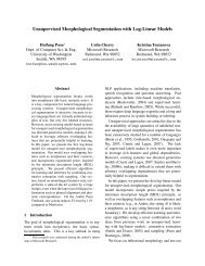
y regularizing a classifier toward equal weights, a supervised predictor outperforms theunsupervised approach after only ten examples, and does as well with 1000 examples as thestandard classifier does with 100,000.Section 4.2 first describes a general multi-class SVM. We call the base vector of informationused by the SVM the attributes. A standard multi-class SVM creates features forthe cross-product of attributes and classes. E.g., the attribute COUNT(Russia during 1997) isnot only a feature for predicting the preposition during, but also for predicting the 33 otherprepositions. The SVM must therefore learn to disregard many irrelevant features. We observethat this is not necessary, and develop an SVM that only uses the relevant attributesin the score for each class. Building on this efficient framework, we incorporate varianceregularization into the SVM’s quadratic program.We apply our algorithms to the three tasks studied in Chapter 3: preposition selection,context-sensitive spelling correction, and non-referential pronoun detection. We reproducethe Chapter 3 results using a multi-class SVM. Our new models achieve much better accuracywith fewer training examples. We also exceed the accuracy of a reasonable alternativetechnique for increasing the learning rate: including the output of the unsupervised systemas a feature in the classifier.Variance regularization is an elegant addition to the suite of methods in NLP that improveperformance when access to labeled data is limited. Section 4.5 discusses somerelated approaches. While we motivate our algorithm as a way to learn better weightswhen the features are counts from an auxiliary corpus, there are other potential uses ofour method. We outline some of these in Section 4.6, and note other directions for futureresearch.4.2 Three Multi-Class SVM ModelsWe describe three max-margin multi-class classifiers and their corresponding quadratic programs.Although we describe linear SVMs, they can be extended to nonlinear cases in thestandard way by writing the optimal function as a linear combination of kernel functionsover the input examples.In each case, after providing the general technique, we relate the approach to ourmotivating application: learning weights for count features in a discriminative web-scaleN-gram model.4.2.1 Standard Multi-Class SVMWe define a K-class SVM following [Crammer and Singer, 2001]. This is a generalizationof binary SVMs [Cortes and Vapnik, 1995]. We have a set {(¯x 1 ,y 1 ),...,(¯x M ,y M )} of Mtraining examples. Each ¯x is an N-dimensional attribute vector, and y ∈ {1,...,K} areclasses. A classifier, H, maps an attribute vector, ¯x, to a class, y. H is parameterized by aK-by-N matrix of weights, W:H W (¯x) =Kargmaxr=1{ ¯W r · ¯x} (4.1)where ¯W r is the rth row of W. That is, the predicted label is the index of the row of Wthat has the highest inner-product with the attributes, ¯x.57