Large-Scale Semi-Supervised Learning for Natural Language ...

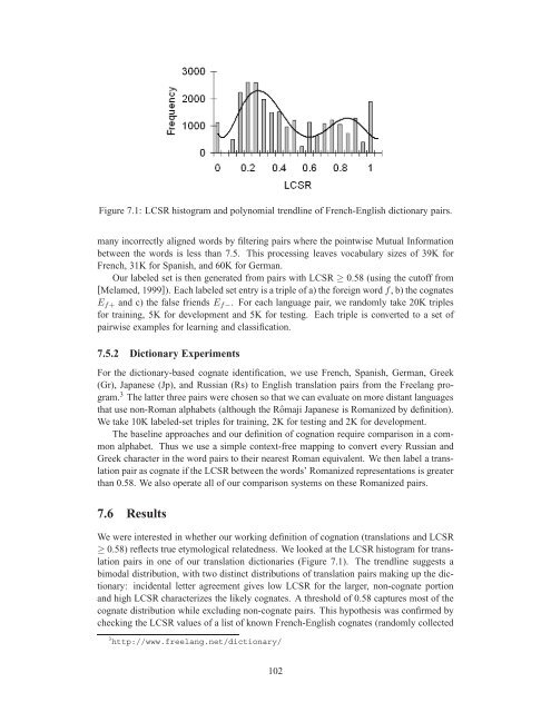
Figure 7.1: LCSR histogram and polynomial trendline of French-English dictionary pairs.many incorrectly aligned words by filtering pairs where the pointwise Mutual Informationbetween the words is less than 7.5. This processing leaves vocabulary sizes of 39K forFrench, 31K for Spanish, and 60K for German.Our labeled set is then generated from pairs with LCSR ≥ 0.58 (using the cutoff from[Melamed, 1999]). Each labeled set entry is a triple of a) the foreign wordf, b) the cognatesE f+ and c) the false friends E f− . For each language pair, we randomly take 20K triplesfor training, 5K for development and 5K for testing. Each triple is converted to a set ofpairwise examples for learning and classification.7.5.2 Dictionary ExperimentsFor the dictionary-based cognate identification, we use French, Spanish, German, Greek(Gr), Japanese (Jp), and Russian (Rs) to English translation pairs from the Freelang program.3 The latter three pairs were chosen so that we can evaluate on more distant languagesthat use non-Roman alphabets (although the Rômaji Japanese is Romanized by definition).We take 10K labeled-set triples for training, 2K for testing and 2K for development.The baseline approaches and our definition of cognation require comparison in a commonalphabet. Thus we use a simple context-free mapping to convert every Russian andGreek character in the word pairs to their nearest Roman equivalent. We then label a translationpair as cognate if the LCSR between the words’ Romanized representations is greaterthan 0.58. We also operate all of our comparison systems on these Romanized pairs.7.6 ResultsWe were interested in whether our working definition of cognation (translations and LCSR≥ 0.58) reflects true etymological relatedness. We looked at the LCSR histogram for translationpairs in one of our translation dictionaries (Figure 7.1). The trendline suggests abimodal distribution, with two distinct distributions of translation pairs making up the dictionary:incidental letter agreement gives low LCSR for the larger, non-cognate portionand high LCSR characterizes the likely cognates. A threshold of 0.58 captures most of thecognate distribution while excluding non-cognate pairs. This hypothesis was confirmed bychecking the LCSR values of a list of known French-English cognates (randomly collected3 http://www.freelang.net/dictionary/102