epidemiology final exam review

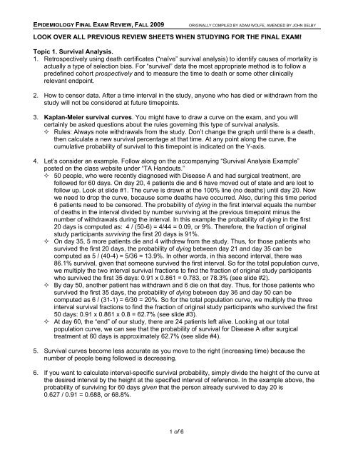
EPIDEMIOLOGY FINAL EXAM REVIEW, FALL 2009ORIGINALLY COMPILED BY ADAM WOLFE, AMENDED BY JOHN SELBYLOOK OVER ALL PREVIOUS REVIEW SHEETS WHEN STUDYING FOR THE FINAL EXAM!Topic 1. Survival Analysis.1. Retrospectively using death certificates (“naïve” survival analysis) to identify causes of mortality isactually a type of selection bias. For “survival” data the most appropriate method is to follow apredefined cohort prospectively and to measure the time to death or some other clinicallyrelevant endpoint.2. How to censor data. After a time interval in the study, anyone who has died or withdrawn from thestudy will not be considered at future timepoints.3. Kaplan-Meier survival curves. You might have to draw a curve on the exam, and you willcertainly be asked questions about the rules governing this type of survival analysis. Rules: Always note withdrawals from the study. Don’t change the graph until there is a death,then calculate a new survival percentage at that time. At any point along the curve, thecumulative probability of survival to this timepoint is indicated on the Y-axis.4. Let’s consider an example. Follow along on the accompanying “Survival Analysis Example”posted on the class website under “TA Handouts.” 50 people, who were recently diagnosed with Disease A and had surgical treatment, arefollowed for 60 days. On day 20, 4 patients die and 6 have moved out of state and are lost tofollow up. Look at slide #1. The curve is drawn at the 100% line (no deaths) until day 20. Nowwe need to drop the curve, because some deaths have occurred. Also, during this time period6 patients need to be censored. The probability of dying in the first interval equals the numberof deaths in the interval divided by number surviving at the previous timepoint minus thenumber of withdrawals during the interval. In this example the probability of dying in the first20 days is computed as: 4 / (50-6) = 4/44 = 0.09, or 9%. Therefore, the fraction of originalstudy participants surviving the first 20 days is 91%. On day 35, 5 more patients die and 4 withdrew from the study. Thus, for those patients whosurvived the first 20 days, the probability of dying between day 21 and day 35 can becomputed as 5 / (40-4) = 5/36 = 13.9%. In other words, in this second interval, there was86.1% survival, given that someone survived the first interval. So for the total population curve,we multiply the two interval survival fractions to find the fraction of original study participantswho survived the first 35 days: 0.91 x 0.861 = 0.783, or 78.3% (see slide #2). By day 50, another patient has withdrawn and 6 die on that day. Thus, for those patients whosurvived the first 35 days, the probability of dying between day 36 and day 50 can becomputed as 6 / (31-1) = 6/30 = 20%. So for the total population curve, we multiply the threeinterval survival fractions to find the fraction of original study participants who survived the first50 days: 0.91 x 0.861 x 0.8 = 62.7% (see slide #3). At day 60, the “end” of our study, there are 24 patients left alive. Looking at our totalpopulation curve, we can see that the probability of survival for Disease A after surgicaltreatment at 60 days is approximately 62.7% (see slide #4).5. Survival curves become less accurate as you move to the right (increasing time) because thenumber of people being followed is decreasing.6. If you want to calculate interval-specific survival probability, simply divide the height of the curve atthe desired interval by the height at the specified interval of reference. In the example above, theprobability of surviving for 60 days given that the person already survived to day 20 is0.627 / 0.91 = 0.688, or 68.8%.1 of 6

EPIDEMIOLOGY FINAL EXAM REVIEW, FALL 2009ORIGINALLY COMPILED BY ADAM WOLFE, AMENDED BY JOHN SELBYTopic 2. Interpreting Medical Tests.This lecture has some very high yield information for your Step I exam.Be sure you understand the mathematical and semantic definitions of the bolded terms below.1. Remember our table of test results versus disease? You need to be able to calculate the followingparameters from a 2x2 table: False positive rate = b/(b+d) False negative rate = c/(a+c) Sensitivity = a/(a+c); the probability of having a positive test result if you have the disease. Specificity = d/(b+d); the probability of having a negative test result if you do not have thedisease. Positive predictive value (also called post-test probability of a positive test) is not the sameas sensitivity! It takes the prevalence of the disease into account. It answers the question, howlikely is someone from the population at large to have the disease, given a positive test result?Mathematically, it is calculated as true positives divided by all positive tests. Negative predictive value is not the same as specificity! How likely is someone from thepopulation at large not to have the disease, given a negative test? Mathematically, it iscalculated as true negatives divided by all negative tests.“Reality” or “Truth” “Reality” or “Truth” TotalsDisease (+) Disease (-)Test (+) aba+bCorrect result! False positive!Test (-)cdc+dFalse negative! Correct result!Totals a+c b+d a+b+c+d2. It is unlikely that a single test can have 100% sensitivity and specificity. If it does, it’s probably nota great test. Look at Dr. Gayed’s slides from this lecture to see what happens when you selectdifferent sensitivity and specificity values for a test on a graph of population values. Receiver-Operating Characteristic (ROC) curve plots the change in sensitivity vs.false-positive rate (1-specificity) for a typical test. Note that as we increase the sensitivity ofthe test, the specificity decreases. Picking the “best” combination of sensitivity and specificityis often challenging, and depends on how many false positives/negatives you are willing totolerate. A test is considered better if the area under the ROC curve is greater. Now consider a disease that is not very prevalent. How do we interpret false positives andnegatives when testing for it? This is why we have predictive values.3. Predictive values again. Just like case-control studies don’t tell us anything about populationstatistics, a case-control table cannot be used on its own to establish positive and negativepredictive values. We need prevalence (also called pre-test probability) of the disease and mustadjust the case-control table to reflect a proportional population. Consider this table from lecture:“Reality” or “Truth” “Reality” or “Truth” TotalsDisease (+) Disease (-)Test (+) 95 8 103Test (-) 5 92 97Totals 100 100 200 Sensitivity = 95%, specificity = 92%. If you were given this case-control table and asked tocalculate PPV and NPV, you would not have enough information to do so! Do not be temptedto calculate it as 95/103 (92%)! We do not know prevalence yet. Now let’s say the prevalence of the disease is 10% in our population. We could adjust thistable, taking into account the sensitivity and specificity values above, to reflect a hypotheticalpopulation of 1000 people:2 of 6

EPIDEMIOLOGY FINAL EXAM REVIEW, FALL 2009ORIGINALLY COMPILED BY ADAM WOLFE, AMENDED BY JOHN SELBY“Reality” or “Truth” “Reality” or “Truth” TotalsDisease (+) Disease (-)Test (+) 95 72 167Test (-) 5 828 833Totals 100 900 1000 If you don’t understand what was done here, re-calculate the sensitivity and specificity values.You will see that they are still 95% and 92%. All we did was set up a population with 10%disease prevalence (100/1000 disease +, 900/1000 disease -). PPV = true positives/all positive tests = 95/167 = 57%. NPV = true negatives/all negative tests = 828/833 = 99%.4. Likelihood ratios. LR+ is the ratio of probabilities of a true positive to false positive test result, orsensitivity / (1-specificity). LR- is the ratio of probabilities of a false negative to true negative testresult, or (1-sensitivity) / specificity. Note that both types of likelihood ratio are predicting thelikelihood of having the disease. Look back at the table above. The LR+ would be sensitivity/(1-specificity) = 0.95/(1-0.92) =0.95/0.08 = 11.9, so if I have a positive test I am roughly 12x more likely to have the diseasethan to not have the disease. LR- would be (1-sensitivity)/specificity = 0.05/0.92 = 0.054, so if I have a negative test I amalmost 20x less likely to have the disease.5. Dr. Gayed’s mnemonics. SpIN: A test with a high specificity can be used to “rule-IN” a disease, because positive resultsare more likely to be true positives than false. SnOUT: A test with a high sensitivity can be used to “rule-OUT” disease, because negativeresults are more likely to be true negatives than false.6. Combination tests Serial testing: perform multiple tests in a sequence as a cost-saving measure. If any test isnegative, stop testing. All must be positive to diagnose the patient. This method increasesthe specificity above all of the individual tests, but lowers sensitivity below all of theindividual tests. 1-Sp (combination) = (1-Sp) x (1-Sp) x... for each individual test.Sn (combination) = Sn x Sn x... for each individual test. Parallel testing. Perform multiple tests simultaneously. If any one is positive, diagnosis ismade. Increases sensitivity above all of the individual tests, but lowers specificity below all ofthe individual tests. 1-Sn (combination) = (1-Sn) x (1-Sn) x... for each individual test. Sp(combination) = Sp x Sp x... for each individual test. Used to rule out serious but treatableconditions, such as myocardial infarction.Topic 3. Screening.1. When do we screen for a disease? We should screen for a disease when the disease is common,serious, treatable, slow to develop symptoms, and treatable in the asymptomatic condition, i.e.,superior outcomes if treated when asymptomatic versus treatment when symptomatic. The testshould have high predictive values, be inexpensive, and something the patient and physician arewilling to perform. Ideally, a high sensitivity would be great, but it’s more important to have a highspecificity if the disease is not too common (less chance of false positives).2. More biases: Lead-Time Bias. We diagnose a disease based on when symptoms appear, and measure lifeexpectancy. Now we diagnose based on a screening test (pre-symptoms), and measure lifeexpectancy. Since our screening test found the disease earlier in the disease process, thescreened patients appear to live longer, simply because of the early diagnosis! This makes usthink that the screening prolonged their lives, even if the treatment had no effect.3 of 6

EPIDEMIOLOGY FINAL EXAM REVIEW, FALL 2009ORIGINALLY COMPILED BY ADAM WOLFE, AMENDED BY JOHN SELBY Length-Time Bias. Similar to above, this bias makes us think that screening prolongs life,even if the treatment is ineffective. In this case, our screening test detects patients who haveslow-progressing variants of the disease. Fast-progressing patients become symptomaticquickly, and also die quicker, but if we just lump everyone together it looks like the screeningprolonged survival. Compliance (Volunteer) Bias. Same as from a previous lecture. People who volunteer formedical testing (including screening) tend to take better care of themselves overall and aremore likely to comply with treatment. As a screening population, they appear to do better thanthe general population even if the early treatment is not very effective.Topic 4. Case study: Screening for HIV. This case study reviews all of the issues described aboveunder “Screening.”Topic 5. Decision Analysis. I strongly recommend that you look back over Dr. Gayed’s lecture slidesand attempt to draw out the decision tree for the decision analysis assignment he provided in class.While you may not be asked to draw a decision analysis tree for your exam, you will probably beasked to analyze one and should understand what all of the symbols and numbers represent in acompleted tree.1. You are given a number of interventions for a particular problem, and the probabilities of certainoutcomes from each intervention. These outcomes can be things such as “cure,” “improvement,”“worsening,” “death,” etc. If an intervention is actually a test of some kind, the probabilities of eachoutcome (based on predictive values) are provided.2. Start your analysis by drawing a tree with each intervention/test the subject might choose.The branches of the tree, then, represent every possible combination of interventions andoutcomes. Use boxes to indicate places where the subject can make a decision, circles to indicateevents determined by chance occurrences, and ovals to indicate endpoints.3. At each branch point, enter the probabilities for each new branch.4. At each endpoint, assign “utilities.” These can be concrete values, such as life expectancies, orarbitrary values, such as the patient’s perceived quality of life.5. Fold back the tree. This means that you start at the endpoints, and multiply each endpoint utilityby the probability on that branch (going back to the last chance or decision point). Now addtogether all of these products (“weighted utilities”) for the node. This sum is the overall utility of thenode (either a decision or chance node). Now repeat this process at each node, working to thebase of the tree. You will ultimately have a weighted utility for the very first decision point, whichrepresents a suggestion of which choice represents the most likely “good” outcome for the patient.6. Sensitivity analysis. What if our arbitrary utilities biased our ultimate decision? You can go back toyour utilities, and adjust the numbers. For example, if the patient originally gave a utility of 1.0 forthe outcome “improvement” and utility 0.5 for the outcome “no change,” try adjusting the“no change” utility to 0.75, fold back the tree again, and see if the decision recommendationchanges. The larger of a change in utilities required to affect a change in the decisionrecommendation, the more robust the tree was. Note: “sensitivity analysis” in this context has nothing to do with “sensitivity” of diagnostic testsdiscussed in another lecture!4 of 6

EPIDEMIOLOGY FINAL EXAM REVIEW, FALL 2009ORIGINALLY COMPILED BY ADAM WOLFE, AMENDED BY JOHN SELBYTopic 6. Making sense of multiple studies.1. The more tests you run indiscriminately on patients, the more likely there will be some abnormalfinding. Does this mean that everyone has something wrong with them? Probably not. Rememberfrom the statistics lecture that most lab tests determine a “normal” result based on an interval thatincludes the middle 95% of the general population. That means that on any one test there is a 5%chance that a normal person has a value outside of the “normal” range for the test. If yourandomly test someone for 20 serum markers all at once, it is very likely that you will find an“abnormality,” even though nothing is wrong.2. For the reason just explained, it is important to have an indication to order a test on a patient.The indication represents an increased suspicion or pretest probability on the clinician’s part,increasing the likelihood ratio that the test will have a correct and useful result.3. During a clinical trial, each time you check patient status mid-trial you actually raise your α value(reducing the statistical significance of your findings). Why? Because each time you “look in” onthe trial results, it’s like performing another “test” and random variation from test to test increasesyour probability of finding a result based purely on chance. This phenomenon is calledα consumption. O’brien-Fleming rules are used in clinical trials to determine threshold p values fordeciding whether or not to terminate the trial depending on the number of times you “look in” onthe data.4. Causality between an exposure and an outcome: Strength of association: a higher relative risk makes the causality easier to detect/prove. Consistency: multiple studies with different populations and test methods that detect the sameassociation between exposure and outcome is strong evidence for causality. Temporality: exposure must precede outcome. Dose-response: more exposure increases likelihood or severity of the outcome. Reversibility: discontinuing exposure reduces risk of the outcome. Biologic plausibility: a “scientific” explanation how the exposure causes the outcome. In manyinstances, biological plausibility follows the establishment of causality. Think back to thestudies that linked cigarette smoking to lung cancer. Even today, the pathophysiologicalmechanisms underlying the relationship are not completely known. Specificity: one cause leads to one effect. Analogy: this exposure-disease relationship resembles a different one that is well-established.5. What are the types of research that establish a cause-effect relationship? From worst to best:case report, case series, case-control, cohort study, clinical trial.6. Meta-Analysis. A meta-analysis pools the results and observations from multiple studies in theliterature to try and improve the statistics of the smaller studies. Bigger N = better combinedpower. However, any biases and confounding factors present in those studies are still present.All the meta-analysis does is to help us form a hypothesis for the design of a larger clinical study,with better power and narrower confidence intervals. Publication Bias. The meta-analysis will only include studies that got published. However,negative results are much less frequently published than positive ones. So trials that “failed”might not make it into the meta-analysis. We can check for this and other biases by drawing a“funnel plot” of all of the constituent studies of the meta-analysis. The funnel plot features avertical axis relating to the power of the studies and a horizontal axis showing the observedeffect in each trial (“effect” might be odds ratio, etc.). A meta-analysis containing few biasesshould show a funneling of studies as their powers drop. In other words, the low-power studieswill scatter about the summary odds ratio symmetrically. If the plot is asymmetric, andlow-power studies all fall to one side or the other of the summary odds ratio, then we suspect5 of 6

EPIDEMIOLOGY FINAL EXAM REVIEW, FALL 2009ORIGINALLY COMPILED BY ADAM WOLFE, AMENDED BY JOHN SELBYbiases, such as publication bias, may have weighted the types of studies that appeared in themeta-analysis and therefore we should not trust its conclusions.7. Make sure when you read an article to examine exclusion criteria. How many patients wereoriginally enrolled? How many were excluded based on predetermined criteria? How many wererandomized into each arm of the trial? How many dropped out during the trial?6 of 6