National Digital Forecast Database (NDFD) Tkdegrib and ... - NOAA

National Digital Forecast Database (NDFD) Tkdegrib and GRIB2 

DataDownload and ImgGen Tool Tutorial 

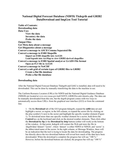
Table of Contents: 

Downloading data 

Data Uses 

View the data 

Inventory the data 

Probe the data 

Output Files 

Get Meta data about a message 

Get Diagnostics about a message 

Convert a message to ASCII Comma Separated file 

Convert a message to ESRI Shapefile 

Import an ESRI shapefile into ArcGIS 

Load legends into ArcMap to view GRIB2-derived shapefiles 

Convert a message to ESRI Spatial analyst or GrADS File format 

Open an FLT file in ArcGIS 

Convert a message to NetCDF 

Convert a sub grid of certain types of GRIB2 files to GRIB2 

Create a flat file database 

Probe a flat file database 

Downloading data 

After the National Digital Forecast Database Tkdegrib and Grib2 is installed, data will need to be 

downloaded. This can be done by manually transferring the data to the machine in use. 

The Uniform Resource Locators (URLs) for NDFD and the National Digital Guidance Database 

(NDGD) are located at www.nws.noaa.gov/mdl/NDFD_GRIB2Decoder/dataloc.php. The data can 

be manually downloaded from this site, but the degrib program comes with two ways to 

automatically access those URLs: from the graphical user interface (GUI) or from the command 

line. 

1. On the Download tab of the GUI program tkdegrib, expand the ndfd data set and 

highlight a sector, or region, in the left column, or expand the sector file by clicking on 

the plus symbol (+) next to the sector and highlight the specific weather element (Figure 

1). To download more than one specific weather element for a sector, hold down the 

Control key on the keyboard and click on the desired weather elements. Then click either 

the Download by ftp or the Download by http buttons (either will work) at the bottom 

of the window. At that point, tkdegrib will contact the Web and store the file in 

/degrib/data/’dataset’/’sector’, where ‘dataset’ is either NDFD or NDGD, and ‘sector’ is 

the abbreviated name of the sector. In the right column, or Message Window, there will 

be an indication that the tool is trying to locate the data for downloading. The progress 

bar directly above the two download buttons will reveal how much of the data have been 

downloaded. When the download is complete the progress bar will say “100 %.” 

However, before the download buttons are clicked, the progress bar will say “100 %”

DataDownload and ImgGen Tool Tutorial Page 2 

(even if no data have been downloaded), but then once the buttons are clicked it will start 

at “0 %” (see Figure 1). 

Note: The abbreviations for the individual weather elements are as follows: maxt 

(maximum temperature), mint (minimum temperature), pop12 (probability of 

precipitation), qpf (quantitative precipitation forecast), sky (percent of total cloud 

coverage), snow (total snowfall), td (dew point temperature), waveh (wave height), wdir 

(wind direction from which it is blowing), wspd (wind speed), and wx (weather string). 

2. From a command line or a script (Note: in Microsoft Windows, replace /degrib/ with 

c:\ndfd\degrib16\): 

• /degrib/bin/tcldegrib web.tcl ndfd midatlan,all should get from the ndfd data set 

all weather elements found in the midatlan sector. 

• /degrib/bin/tcldegrib web.tcl ndfd conus,maxt,mint should get from the ndfd data 

set the maxt and mint weather elements found in the conus sector. 

• /degrib/bin/tcldegrib web.tcl ndgd conus,ozone01 should get from the ndgd data 

set the ozone01 forecast found in the conus sector. 

Figure 1: In the Download tab, the Eastern Great Lakes sector has been 

expanded. In this example, the user is only interested in the Wind Direction 

weather element, so the Wind Direction is highlighted. Then the user will click 

on either Download by ftp or Download by http. Notice that the progress bar 

says “100 %” before anything has been downloaded.


Data Uses 

View the data 

To get an idea of what the data look like before conversion to other formats (including .shp, .csv, 

.flt), the user can view the data to see if they are desirable. On MS-Windows, use tkdegrib with 

superImageGen and htmlmaker to create images (.png) and a means of browsing those images 

with Microsoft (MS) Internet Explorer. 

1. In the GUI tkdegrib: 

The images can include all the weather elements in a whole sector, or just one or a few 

selected weather elements within a sector. To view all the weather elements within a 

sector, click on the Download tab, highlight the desired sector in the left column, and 

click the Generate Images button at the bottom of the window. To view specific weather 

elements, expand the sector of choice in the left column and click on the desired weather 

element. To choose more than one, hold down the Control key on the keyboard and click 

on more than one weather element. When all desired weather elements are highlighted, 

click on the Generate Images button. That will cause tkdegrib to convert the selected 

forecasts to mosaic (*.tlf) files. The .tlf file, which is similar to the .flt file, contains the 

grid in an NxM 4 byte (octet) float file, which starts generating the image in the lower left 

corner, traverses a row, then starts again on the left. Use .tlf files when using imageGen 

(otherwise use .flt files). Then tkdegrib calls superImageGen to read the mosaic (*.tlf) 

files and draw the images. Next htmlmaker is called to create html pages to help view the 

images, and finally Internet Explorer is called to browse the html. 

In the Internet Explorer window there will be a chart on the left with the time period for 

which the weather is forecasted and columns of each weather element. To the left of the 

chart there will be a map of the generated sector image. When the cursor is placed on a 

weather element for a given time period, that weather element will be depicted on the 

map of the sector (Figure 2). 

Note 1: Unfortunately, superImageGen is an executable that only works on Windows 

machines. 

Note 2: The Image folder on the local drive should be cleared out often if images are 

generated frequently. Old images are not overridden and will use storage space on the 

machine. 

Note 3: Some versions of Internet Explorer have an active content protector to 

discourage pop-ups. Disabling this protector will allow the active images to be viewed. 

2. From the command line: 

Currently there is no way to perform this function from the command line.


Figure 2: The image above shows the weather forecast for the generated weather element for 

the Southern Plains. The chart on the left reveals the weather forecast for the day the image 

was generated through the following Tuesday. The columns include maximum and minimum 

temperature for the day (Low/High Temp), probability of precipitation (pop12), temperature 

and wind direction (Temp/Wind), dew point temperature (Dewpoint), and percent of total 

cloud coverage (sky). The cursor is pointed to Wednesday’s temperature and wind direction at 

12:00 p.m., which is depicted in the image on the right. 

Inventory the data 

To see what messages are inside a GRIB file, use degrib to inventory it. 


Click on the GIS tab, and browse through the files in the upper left corner of the window 

for the downloaded file of choice. Double-click on a specific weather element in the top 

right corner, and it should fill out the inventory chart in the bottom half of the window 

with the following: message number, a short version of the variable name, a long version 

of the variable name, the level or surface (i.e., the level above the surface of the Earth 

where the data were forecasted), the reference date (the time at which the forecast was


created), the valid time and date (the time at which the forecast will be true), and the 

difference between the valid time and the reference time (Figure 3). For example, in 

Figure 3, the highlighted message number (7.0) is for temperature, or temp. The data 

were collected at ground level (Level) on May 10, 2005, at 12:00 p.m. (Ref. Date). The 

time the forecast will be true (Valid date) is at 9:00 a.m. on May 11, 2005, which is 21 

hours from the time the forecast was made (Val-Ref). 

Figure 3: In this example, the user wants to inventory the data for the temperature of the Northeast 

(neast). In the top left window, the Northeast sector has been expanded and the individual weather 

elements can be seen in the top right window. The temp, or the temperature, element was doubleclicked 

and each variable for percent of total cloud coverage was revealed in the inventory chart in the 

mid-section of the window. The area within the red box changes depending on which file type is 

selected. 


/degrib/bin/degrib “GRIB file” -I 

where “GRIB file” is replaced with the name of the downloaded GRIB file.


This should print out the message number, which byte it starts on, the GRIB version, the 

variable name (both short and long forms of it), the level or surface, the reference time, 

the valid time, and the forecast projection. 

Probe the data 

To get a better feel for the data, use degrib to probe the file at a given latitude/longitude point, or 

a set of points in a point file. 


Currently there is no way to perform this function from the GUI. 


/degrib/bin/degrib “GRIB file” -P -pnt 38,-76 

/degrib/bin/degrib “GRIB file” -P -pntFile “foo.txt” 

where “GRIB file” is replaced with the name of the downloaded GRIB file, and “foo.txt” 

is replaced with a file that contains station ID, lat, lon. 

This should read the file, and extract each message in the file. Then it will either 

bilinearally interpolate to the given latitude/longitude point, or find the nearest neighbor, 

and output that data to stdout. See the “degrib Man Page” (particularly the “PROBE 

OPTIONS” section) for more details. 

Output files 

Each time a file is generated there are three options to choose where the generated files are 

stored: in the OUTPUT Filename box, manually type the desired location of the generated file; 

browse to a desired file location; or click the Recommend button to have tkdegrib choose one. If 

tkdegrib chooses the file, it will output the file in the local drive in the ndfd/degrib16/output 

folder. In the output folder, all the sectors will be listed. The downloaded file will be in the sector 

corresponding to the downloaded data. Each file generated is named according to the specific 

weather element and valid date of forecast. For example, in Figure 3 the OUTPUT Filename is 

c:/ndfd/degrib16/output/neast/200505110900_t.shp, where the forecast is for the temperature (_t) 

of the North East sector at time 9:00 a.m. (0900) on May 11, 2005 (20050511). The type of file 

being generated is a shapefile (.shp). 

Get metadata about a message 

To get “metadata” or information describing a GRIB message, use degrib to create a .txt file. 

Among the “metadata” will be the maximum value, the minimum value, the number of missing 

values detected, etc. 


Each time a message is converted from a file, the GUI automatically creates a .txt file that 

contains the metadata. To convert a file, click on the GIS tab, and browse for the 

downloaded file of interest. Double-click the specific weather element in the top right 

window, and it will fill out the inventory chart in the bottom half of the window. 

Highlight the message in the inventory chart, and click the Choose File Type button at 

the bottom left of the window. Select a file type from the drop-down menu. Then 

manually type the name into OUTPUT Filename dialog box or click Recommend to 

have tkdegrib choose one (see “Output files” above). The tool will also generate a text


file that will be in the same location. The default values for the box in the bottom right 

corner for Round data to and Units (when possible) can be accepted or changed, 

depending on personal preferences. The values for both Force Major Earth Axis and 

Force Minor Earth Axis are more advanced options and should be left as 0 for general 

purposes. Then click the Generate file button at the bottom left side of the window. 

Note: The “Round data to” value will show its default when the Recommend button is 

selected. Most the weather elements will default as 0; the exceptions are snow and 

waveh, which will default as 1, and qpf, which will default as 2. 


/degrib/bin/degrib “GRIB file” -C -msg 1 

/degrib/bin/degrib “GRIB file” -C -msg all 

/degrib/bin/degrib “GRIB file” -C -Met -msg 2 -out message2.txt 

where “GRIB file” is replaced with the name of the downloaded GRIB file. 

This should read the file and extract the requested messages. The -Met option (on by 

default) tells it to create a .txt file with the metadata. To turn off the meta file option, use 

-nMet. See the “degrib Man Page” (particularly the “CONVERT OPTIONS” section) for 

more details. 

Get diagnostics about a message 

To get some diagnostics about the message before it has been parsed by the code, create an .is0 

file. This can be useful for diagnosing packing and unpacking routines, but the WMO GRIB2 

Document FM92-X11 GRIB is needed to understand the results. 




/degrib/bin/degrib “GRIB file” -C -nMet -IS0 -msg 1 

/degrib/bin/degrib "GRIB file" -C -IS0 -msg all 


Convert a message to an ASCII comma-separated file 

Use degrib to convert a given message to a .csv file, which is a comma delimited ASCII file that 

contains x, y, lat, lon, and value line for each cell in the grid. This file can be imported into Excel 

(limited to the first 65,536 lines), or read by other files to populate an SQL database. 


Click on the GIS tab, and browse for the downloaded file. Double-click on the specific 

weather element in the top right corner, and it will fill out the chart in the mid-section of 

the window. Click on the desired message in the inventory chart. Click the Choose File 

Type button at the bottom left corner of the window and choose CSV from the dropdown 

menu. In Figure 3 the red box in the bottom left corner will no longer have options 

for types of shapefiles. Instead there will be an option to include missing values in the 

generated data. This box can be selected if preferred. Manually type the output file name 

into the OUTPUT Filename dialog box or click Recommend to have tkdegrib choose 

one (see “Output files”). The default values for the box in the bottom right corner for


Round data to and Units (when possible) can be accepted or changed, depending on 

personal preferences (see note under “Get Metadata about a message”). The values for 

both Force Major Earth Axis and Force Minor Earth Axis are more advanced options and 

should be left as 0 for general purposes. Then click the Generate .csv file button at the 

bottom of the window. This creates a comma-delimited text file which can be imported 

into a spreadsheet. 


/degrib/bin/degrib “GRIB file” -C -msg 1 -Csv 

/degrib/bin/degrib “GRIB file” -C -msg all -nMet -Csv 

where “GRIB file” is replaced with the name of a downloaded GRIB file. 

This should read the file and extract the requested messages. The CSV option tells it to 

create the .csv file. See the “degrib Man Page” (particularly the “CONVERT OPTIONS” 

section) for more details. 

Convert a message to ESRI shapefile 

Use degrib to convert a given message to three different types of ESRI shapefiles: point, small 

polygon, or large polygon. A point contains the latitude and longitude and is the centroid of each 

grid cell (Figure 4A). A small polygon is a small five-vertex polygon that represents the value of 

each grid cell (Figure 4B). A large polygon represents the polygons dissolved by like attributes, 

so all like values are grouped together into one large polygon (Figure 4C). Polygons give areal 

coverage. Large polygons are smaller files and they are more manageable than small polygons. 


Click on the GIS tab and browse for the downloaded file in the top left corner of the 

window. Double-click on a specific weather element in the top right corner, and it should 

fill out the inventory chart below. Select the desired message in the inventory chart. Then 

click on the Choose File Type button at the bottom left corner of the window and choose 

SHP. Then manually type the output file name into the OUTPUT Filename dialog box or 

click the Recommend button to have tkdegrib choose one (see “Output files”). Now 

choose the Type of .shp file (point, small polygon, or large polygon). Check the box for 

Verbose .shp file if the values for latitude, longitude, and X and Y are needed (Figure 

5A). A non-verbose shapefile will generate point identification and data, but will not 

generate the latitude, longitude, and X and Y (Figure 5B). The default values for the box 

in the bottom right corner for Round data to and Units (when possible) can be accepted or 

changed, depending on personal preferences (see note under “Get Metadata about a 

message”). The values for both Force Major Earth Axis and Force Minor Earth Axis are 

more advanced options and should be left as 0 for general purposes. Then click the 

Generate .shp file button at the bottom center of the window. 


/degrib/bin/degrib “GRIB file” -C -msg 1 -Shp -poly 0 


/degrib/bin/degrib “GRIB file” -C -msg 1 -Shp -poly small 


/degrib/bin/degrib “GRIB file” -C -msg 1 -Shp -poly big 

where “GRIB file” is replaced with the name of the downloaded GRIB file.


A. 

C. 

A. B. 

Figure 4: This example is zoomed in on 

the Pacific Northwest sector to show the 

three different types of shapefiles: point 

(A), small polygon (B), and large polygon 

(C). Notice the large polygons have like 

colors merged together. 

Figure 5: A verbose .shp file imports the point identification (POINTID) and data (T, or 

temperature), as well as the X and Y and latitude (LAT) and longitude (LON) (A). A non-verbose 

.shp file only imports the point identification and data (B). 

B.


This should read the file and extract the requested messages. The -Shp option tells it to create the 

.shp file. The -poly 0 says to create a point shapefile, the -poly 1 or -poly small says to create the 

small polygon shapefile, and the -poly 2 or -poly big says to create the “large polygon” shapefile. 

See the “degrib Man Page” (particularly the “CONVERT OPTIONS” section and the “SHP 

SPECIFIC OPTIONS”) for more details. 

Import an ESRI shapefile into ArcGIS 

Open a new window in ArcMap. Click on the 

Add Data button and navigate to the previously 

selected location of generated .shp files (see 

“Output files”). Highlight the file and click the 

Add button (Figure 6). The shapefile will now 

appear in the Display view on the left side of the 

window, and the Map view will appear in the 

right side of the window (Figure 7). Both the 

Display tab or Table of Contents and the Map 

view tab should already be selected. 

Figure 6: In this example, a shapefile for temperature 

in the Northeast sector was generated and placed in 

the neast folder. Navigate to and highlight the 

shapefile. Click the Add button. 

Load legends into ArcMap to view GRIB2-derived shapefiles 

In the Display view there will be a single symbol with a chosen arbitrary color beneath the 

shapefile name (Figure 7). This symbology is applied by default. To keep the legend consistent 

with the legends used on the NDFD Web pages and created in the SuperImageGen tool, a 

predefined legend needs to be loaded. Predefined legends from ArcView 3 are stored as ArcView 

Legend Files or AVL files. 

Double-click on the shapefile in the Display view (or right-click and scroll down to Properties) of 

ArcMap. In the Layer Properties dialog, click on the Symbology tab (Figure 8A). Then click on 

the Import button in the top left corner. In the Import Symbology dialog box, select Import 

symbology definition from an ArcView 3 legend file (*.avl).


Figure 7: After adding the shapefile into ArcMap, the file (200505070900_t) name is 

shown in the Display view on the left, and the map is shown in the Map view on the right. 

The default symbology for ArcMap is one symbol with a single arbitrary color. This 

example shows the Northeast sector as a point shapefile. 

Then click the Browse button and navigate to the /ndfd/degrib16/arcview/ folder. Select the 

/point_legend or /poly_legend, depending on which type of shapefile was generated, highlight the 

individual weather element that the shapefile addresses, and click the Open button (Figure 8B). 

In the Import Symbology dialog box, under What do you want to import select Complete 

symbology definition (Figure 8C). Click OK. Accept the Value Field default value in the Import 

Symbology Matching Dialog box and click OK. In the Layer Properties dialog there should be 

different colors for the symbol and different numbers for the value. Click OK and notice the 

symbology now applied to the shapefile in both the Display view and the Map view (Figure 9).


Figure 8: In the Symbology tab, click 

on Import (A). The legend to import is 

the one for which the weather element 

was downloaded and added into 

ArcMap. The downloaded file is a point 

shapefile, and in this example is 

temperature-specific. Hence, the 

highlighted .avl file below is for a 

temperature-specific point legend (B). 

When the legend file appears in the 

Legend File window, be sure Complete 

symbology definition is selected and 

click OK (C). 

B. 

A. 

C. 

Figure 9: Once the 

NDFD Web page 

standard legend is 

imported into ArcMap, 

the symbology in both 

the Display view and 

the Map view will 

change. Notice the 

difference between this 

figure and Figure 7.


Convert a message to ESRI Spatial Analyst or GrADS file format 

Use degrib to convert a given message to a .flt file. The .flt file consists of N x M floats where N 

and M are the dimensions of the grid. ESRI Spatial Analyst requires the .flt file along with an .hrd 

file. GrADS used the same format except that, in addition to the .flt file, it required a control file 

(.ctl). 


Click on the GIS tab and browse for the downloaded file in the upper left corner of the 

window. Double-click on a specific weather element in the top right corner of the 

window, and it should fill out the inventory chart in the mid-section of the window. Click 

the desired message in the inventory chart. Then click the Choose File Type button and 

choose FLT from the drop-down menu. The options in the red box in Figure 3 will 

change when FLT is selected. In the Grid drop-down menu, choose one of the three 

options: Projected: Original GRIB (which is original map projection); Coverage: Nearest 

Point (which fills out a flat latitude/longitude grid by finding the nearest points to the 

original grid); or Coverage: Bi-Linear (which fills out a flat latitude/longitude grid by 

finding the four surrounding points on the original grid and does a bi-linear 

interpolation). To create the GrADS .ctl file, click on Create GrADS .ctl file. The other 

three options (Start at Upper Left, use NDFD Weather code, and M.S.B. First) are more 

advanced options and do not need to be selected for general purposes. In the OUTPUT 

Filename dialog box, type the output file name or click Recommend to have tkdegrib 

choose one (see “Output files”). The default values for the box in the bottom right corner 

for Round data to and Units (when possible) can be accepted or changed, depending on 

personal preferences (see note under “Get Metadata about a message”). The values for 

both Force Major Earth Axis and Force Minor Earth Axis are more advanced options and 

should be left as 0 for general purposes. Then click the Generate .flt file button at the 

bottom of the window. 

Note 1: In the Grid drop-down menu, Coverage: Bi-Linear should be used with 

continuous data (e.g., temperature), while Coverage: Nearest Point should be used with 

noncontinuous data (e.g., weather type). Nearest point can be used with continuous data, 

but bi-linear cannot be used with noncontinuous data. 

Note 2: When working from a PC, the Grid selection, Projected: Original GRIB, tends to 

take longer. 


/degrib/bin/degrib “GRIB file” -C -msg 1 -Flt 

/degrib/bin/degrib “GRIB file” -C -msg 1 -Flt -Interp –GrADS 

/degrib/bin/degrib “GRIB file” -C -msg 1 -Flt -GrADS 


This should read the file and extract the requested messages. The FLT option tells the 

program to create the .flt file. The -GrADS option says to create the .ctl file. The -Interp 

allows GrADS to work better, since it tells degrib to interpolate the grid to a 

latitude/longitude coverage grid, which saves GrADS from having to do so. See the 

“degrib Man Page” (particularly the “CONVERT OPTIONS” section and the "FLT 

SPECIFIC OPTIONS") for more details. 

For more information on degrib and GrADS go to 

www.nws.noaa.gov/mdl/NDFD_GRIB2Decoder/grads.php.


For information on FORTRAN or C access to .flt files go to 

www.nws.noaa.gov/mdl/NDFD_GRIB2Decoder/flt.php. 

Open an FLT file in ArcGIS 

To open an FLT file in ArcMap, ArcToolbox is needed. Open ArcMap and click on the 

ArcToolbox icon. This will open the ArcToolbox window. Expand the Conversions Tools 

option in the Favorites window. Next, expand the To Raster option. Then double-click on the 

Float to Raster selection (Figure 10A). This will open the Float to Raster window (Figure 10B). 

In the Input floating point raster file box, find the .flt file that was generated from the NDFD 

DataDownload tool and open it. The program should create an Output Raster location. Then click 

OK. This will bring the float file into ArcMap (Figure 11). 

A. 

B. 

Figure 10: In Toolbox, expand Conversion Tools. Then expand To 

Raster and double-click Float to Raster (A). In the Input floating 

point raster file, browse to the generated .flt file. When the .flt file is 

opened in the input window, the output raster box should have an 

output location in it (B). Click OK. 

Convert a message to NetCDF 

Use degrib to convert a given message to a network Common Data Form (NetCDF) file (.nc). For 

more information about the NetCDF format, visit 

http://my.unidata.ucar.edu/content/software/netcdf/index.html. 


Click on the GIS tab and browse for the downloaded file in the upper left corner of the 

window. Double-click on a specific weather element in the top right corner of the 

window, and it should fill out the inventory chart in the mid-section of the window. 

Select the desired message in the inventory chart. Next click the Choose File Type 

button in the bottom left corner of the window. In the file type drop-down menu choose


NetCDF. Then manually type the output file name into the OUTPUT Filename dialog 

box or click the Recommend button to have tkdegrib choose a name (see “Output files”). 

In the red box (refer to Figure 3), accept the default values under This creates a NetCDF 

file using the ‘CF Metadata Convention Ver. 1.0, 28 Oct 2003’.” The default values 

for the box in the bottom right corner for Round data to and Units (when possible) can be 

accepted or changed, depending on personal preferences (see note under “Get Metadata 

about a message”). The values for both Force Major Earth Axis and Force Minor Earth 

Axis are more advanced options and should be left as 0 for general purposes. Then click 

the Generate NetCDF.nc file button at the bottom of the window. 

Figure 11: The generated FLT file needs to be converted to a raster through ArcToolbox before it can 

be viewed in ArcMap. 


/degrib/bin/degrib “GRIB file” -C -msg 1 -NetCDF 1 


This should read the file, and extract the requested messages. The -NetCDF 1 option tells 

the program to create a NetCDF file using degrib's conventions version 1. This attempts 

to use the CF (climate and forcast) convention. See the “degrib Man Page” (particularly 

the “CONVERT OPTIONS” section) for more details.


Convert a sub grid of certain types of GRIB2 files to GRIB2 

Use degrib to get a sub grid of certain types of GRIB2 files. It only works for GRIB2 files that 

were packed using simple pack, complex pack, or complex pack with second order differencing 

(which NDFD uses, but NCEP does not), since those are the only forms that it knows how to 

pack. This cannot be used to convert a message from GRIB1 to GRIB2, because degrib currently 

does not have a mapping of the GRIB1 metadata to GRIB2 metadata. 




/degrib/bin/degrib “GRIB file” -C -msg 1 -Grib2 -lwlf 30,-105 -uprt 40,-85 

where “GRIB file” is replaced with the name of your GRIB file. 

This should read the file and extract the requested messages. The -Grib2 option tells it to 

create a GRIB2 message. The -lwlf 30,-105 tells it to use a subgrid with the lower left 

corner at lon=-105E, lat=30N. The -uprt 40,-85 tells it to use a subgrid with the upper 

right corner at lon=-85E, lat=40N. See the “degrib Man Page” (particularly the 

“CONVERT OPTIONS” section) for more details. 

Create a flat file database 

Use degrib to create a flat file database that is made up of either many .flt files and an index file 

(.ind), or a single cube file (.dat) and an index file (.ind). This is useful for Common Gateway 

Interface (CGI) access to the NDFD, since probing the uncompressed form of the data is faster 

than probing the GRIB2 files. 




/degrib/bin/degrib “GRIB file” -Data -Index simple.ind 

/degrib/bin/degrib “GRIB file” -Data -Index simple.ind -out simple.dat 

where “GRIB file” is replaced with the name of your GRIB file. 

This should read the file, create a new file simple.dat, append each converted grid to 

simple.dat, and create an index file simple.ind. The -Data option tells it to create the 

database, and the -Index simple.ind tells it what to name the index file. The -out 

simple.dat tells it what to name the .dat file. By default it uses the index filename 

replacing the extension with .dat. See the “degrib Man Page” (particularly the 

“DATABASE CREATE OPTIONS” section) for more details. 

Probe a flat file database 

Degrib can be used to probe a flat file database that is made up of either many .flt files and an 

index file (.ind), or a single cube file (.dat) and an index file (.ind). This is useful for CGI access 

to the NDFD, since probing the uncompressed form of the data is faster than probing the GRIB2 

files. 


Currently there is no way to perform this function from the GUI.



/degrib/bin/degrib “index file” -DP -pnt 35,-76 

where “index file” is replaced with the name of the index file (.ind) that was created 

when using the -Data command. 

This should read the index file, figure out where 35,-76 is, open the (.dat) file or the set of 

(.flt) files, jump to and read that cell, and return the results on the command line. See the 

“degrib Man Page” (particularly the “DATABASE PROBE OPTIONS” section) for 

more details.

National Digital Forecast Database (NDFD) Tkdegrib and ... - NOAA

Create successful ePaper yourself

Delete template?

Save as template?