Interactive Computing with Matlab

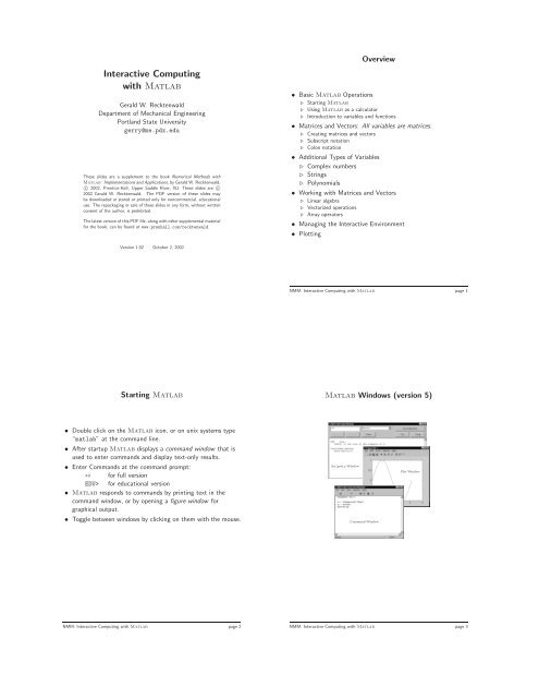
Interactive Computingwith MatlabGerald W. RecktenwaldDepartment of Mechanical EngineeringPortland State Universitygerry@me.pdx.eduThese slides are a supplement to the book Numerical Methods withMatlab: Implementations and Applications, by Gerald W. Recktenwald,c○ 2002, Prentice-Hall, Upper Saddle River, NJ. These slides are c○2002 Gerald W. Recktenwald. The PDF version of these slides maybe downloaded or stored or printed only for noncommercial, educationaluse. The repackaging or sale of these slides in any form, without writtenconsent of the author, is prohibited.The latest version of this PDF file, along with other supplemental materialfor the book, can be found at www.prenhall.com/recktenwald.Overview• Basic Matlab Operations⊲ Starting Matlab⊲ Using Matlab as a calculator⊲ Introduction to variables and functions• Matrices and Vectors: All variables are matrices.⊲ Creating matrices and vectors⊲ Subscript notation⊲ Colon notation• Additional Types of Variables⊲ Complex numbers⊲ Strings⊲ Polynomials• Working with Matrices and Vectors⊲ Linear algebra⊲ Vectorized operations⊲ Array operators• Managing the Interactive Environment• PlottingVersion 1.02 October 2, 2002NMM: Interactive Computing with Matlab page 1Starting MatlabMatlab Windows (version 5)• Double click on the Matlab icon, or on unix systems type“matlab” at the command line.• After startup Matlab displays a command window that isused to enter commands and display text-only results.• Enter Commands at the command prompt:>> for full versionEDU> for educational version• Matlab responds to commands by printing text in thecommand window, or by opening a figure window forgraphical output.• Toggle between windows by clicking on them with the mouse.Helpwin WindowCommand WindowPlot WindowNMM: Interactive Computing with Matlab page 2NMM: Interactive Computing with Matlab page 3

Matlab Workspace (version 6)Matlab as a CalculatorEnter formulas at the command prompt>> 2 + 6 - 4 (press return after ‘‘4’’)ans =4>> ans/2ans =2Or, define and use variables>> a = 5a =5>> b = 6b =6>> c = b/ac =1.2000NMM: Interactive Computing with Matlab page 4NMM: Interactive Computing with Matlab page 5Built-in VariablesBuilt-in Functionspi (= π) and ans are a built-in variables>> pians =3.1416>> sin(ans/4)ans =0.7071Note: There is no “degrees” mode. All angles are measuredin radians.Many standard mathematical functions, such as sin, cos, log,and log10, are built-in>> log(256)ans =5.5452>> log10(256)ans =2.4082>> log2(256)ans =8NMM: Interactive Computing with Matlab page 6NMM: Interactive Computing with Matlab page 7

Looking for FunctionsWays to Get HelpSyntax:lookfor stringsearches first line of function descriptions for “string”.Example:>> lookfor cosine• Use on-line help to request info on a specific function>> help sqrt• The helpwin function opens a separate window for the helpbrowser>> helpwin(’sqrt’)producesACOSACOSHCOSCOSHInverse cosine.Inverse hyperbolic cosine.Cosine.Hyperbolic cosine.• Use lookfor to find functions by keywords>> lookfor functionName• In Matlab version 6 and later the doc function opens theon-line version of the manual. This is very helpful for morecomplex commands.>> doc plotNMM: Interactive Computing with Matlab page 8NMM: Interactive Computing with Matlab page 9On-line HelpSuppress Output with SemicolonSyntax:help functionNameExample:>> help logproducesLOG Natural logarithm.LOG(X) is the natural logarithm of the elements of X.Complex results are produced if X is not positive.See also LOG2, LOG10, EXP, LOGM.Results of intermediate steps can be suppressed with semicolons.Example:Assign values to x, y, and z, but only display the value of z inthe command window:>> x = 5;>> y = sqrt(59);>> z = log(y) + x^0.25z =3.5341Type variable name and omit the semicolon to print the value ofa variable (that is already defined)>> yy =7.6811 ( = log(sqrt(59)) + 5^0.25 )NMM: Interactive Computing with Matlab page 10NMM: Interactive Computing with Matlab page 11

Multiple Statements per LineMatlab Variables NamesUse commas or semicolons to enter more than one statement atonce. Commas allow multiple statements per line withoutsuppressing output.>> a = 5; b = sin(a), c = cosh(a)b =-0.9589c =74.2099Legal variable names:• Begin with one of a–z or A–Z• Have remaining characters chosen from a–z, A–Z, 0–9, or• Have a maximum length of 31 characters• Should not be the name of a built-in variable, built-infunction, or user-defined functionExamples:xxxxxxxxxpipeRadiuswidgets_per_baubblemySummysumNote: mySum and mysum are different variables. Matlab iscase sensitive.NMM: Interactive Computing with Matlab page 12NMM: Interactive Computing with Matlab page 13Built-in Matlab VariablesMatrices and VectorsName Meaningans value of an expression when that expressionis not assigned to a variableeps floating point precisionpi π, (3.141492 ...)realmax largest positive floating point numberrealmin smallest positive floating point numberInf ∞, a number larger than realmax,the result of evaluating 1/0.NaN not a number, the result of evaluating 0/0Rule: Only use built-in variables on the right hand side of anexpression. Reassigning the value of a built-in variablecan create problems with built-in functions.All Matlab variables are matricesA Matlab vector is a matrix with one row or one columnA Matlab scalar is a matrix with one row and one columnOverview of Working with matrices and vectors• Creating vectors:linspace and logspace• Creating matrices:ones, zeros, eye, diag, ...• Subscript notation• Colon notation• VectorizationException: i and j are preassigned to √ −1. Oneorbothofi or j are often reassigned as loop indices. Moreon this laterNMM: Interactive Computing with Matlab page 14NMM: Interactive Computing with Matlab page 15

Creating Matlab VariablesManual EntryMatlab variables are created with an assignment statement>> x = expressionwhere expression is a legal combinations of numerical values,mathematical operators, variables, and function calls thatevaluates to a matrix, vector or scalar.The expression can involve:• Manual entry• Built-in functions that return matrices• Custom (user-written) functions that return matrices• Loading matrices from text files or “mat” filesFor manual entry, the elements in a vector are enclosed in squarebrackets. When creating a row vector, separate elements with aspace.>> v = [7 3 9]v =7 3 9Separate columns with a semicolon>> w = [2; 6; 1]w =261In a matrix, row elements are separated by spaces,and columns are separated by semicolons>> A = [1 2 3; 5 7 11; 13 17 19]A =1 2 35 7 1113 17 19NMM: Interactive Computing with Matlab page 16NMM: Interactive Computing with Matlab page 17Transpose OperatorOverwriting VariablesOnce it is created, a variable can be transformed with otheroperators. The transpose operator converts a row vector to acolumn vector (and vice versa), and it changes the rows of amatrix to columns.>> v = [2 4 1 7]v =2 4 1 7>> v’ans =2417>> A = [1 2 3; 4 5 6; 7 8 9 ]A =1 2 34 5 67 8 9Once a variable has been created, it can be reassigned>> x = 2;>> x = x + 2x =4>> y = [1 2 3 4]y =1 2 3 4>> y = y’y =1234>> A’ans =1 4 72 5 83 6 9NMM: Interactive Computing with Matlab page 18NMM: Interactive Computing with Matlab page 19

Creating vectors with linspaceExample: A Table of Trig FunctionsThe linspace function creates vectors with elements havinguniform linear spacing.Syntax:x = linspace(startValue,endValue)x = linspace(startValue,endValue,nelements)Examples:>> u = linspace(0.0,0.25,5)u =0 0.0625 0.1250 0.1875 0.2500>> u = linspace(0.0,0.25);>> v = linspace(0,9,4)’v =0369>> x = linspace(0,2*pi,6)’; (note transpose)>> y = sin(x);>> z = cos(x);>> [x y z]ans =0 0 1.00001.2566 0.9511 0.30902.5133 0.5878 -0.80903.7699 -0.5878 -0.80905.0265 -0.9511 0.30906.2832 0 1.0000The expressions y = sin(x) and z = cos(x) take advantageof vectorization. If the input to a vectorized function is a vectoror matrix, the output is often a vector or matrix having the sameshape. More on this later.Note: Column vectors are created by appending thetranspose operator to linspaceNMM: Interactive Computing with Matlab page 20NMM: Interactive Computing with Matlab page 21Creating vectors with logspaceFunctions to Create Matrices (1)The logspace function creates vectors with elements havinguniform logarithmic spacing.Syntax:x = logspace(startValue,endValue)x = logspace(startValue,endValue,nelements)creates nelements elements between 10 startValue and10 endValue . The default value of nelements is 100.Example:>> w = logspace(1,4,4)w =10 100 1000 10000NamediageyeonesrandzeroslinspacelogspaceOperation(s) Performedcreate a matrix with a specified diagonal entries,or extract diagonal entries of a matrixcreate an identity matrixcreate a matrix filled with onescreate a matrix filled with random numberscreate a matrix filled with zeroscreate a row vector of linearly spaced elementscreate a row vector of logarithmically spacedelementsNMM: Interactive Computing with Matlab page 22NMM: Interactive Computing with Matlab page 23

Functions to Create Matrices (2)Functions to Create Matrices (3)Use ones and zeros to set intial values of a matrix or vector.Syntax:A = ones(nrows,ncols)A = zeros(nrows,ncols)Examples:>> D = ones(3,3)D =1 1 11 1 11 1 1ones and zeros are also used to create vectors. To do so, seteither nrows or ncols to 1.>> s = ones(1,4)s =1 1 1 1>> t = zeros(3,1)t =000>> E = ones(2,4)E =1 1 1 11 1 1 1NMM: Interactive Computing with Matlab page 24NMM: Interactive Computing with Matlab page 25Functions to Create Matrices (4)Functions to Create Matrices (5)The eye function creates identity matrices of a specified size. Itcan also create non-square matrices with ones on the maindiagonal.Syntax:A = eye(n)A = eye(nrows,ncols)Examples:>> C = eye(5)C =1 0 0 0 00 1 0 0 00 0 1 0 00 0 0 1 00 0 0 0 1>> D = eye(3,5)D =1 0 0 0 00 1 0 0 00 0 1 0 0The diag function can either create a matrix with specifieddiagonal elements, or extract the diagonal elements from amatrixSyntax:A = diag(v)v = diag(A)Example:Use diag to create a matrix>> v = [1 2 3];>> A = diag(v)A =1 0 00 2 00 0 3NMM: Interactive Computing with Matlab page 26NMM: Interactive Computing with Matlab page 27

Functions to Create Matrices (6)Subscript Notation (1)Example:Use diag to extract the diagonal of a matrix>> B = [1:4; 5:8; 9:12]B =1 2 3 45 6 7 89 10 11 12>> w = diag(B)w =1611Note: The action of the diag function depends on thecharacteristics and number of the input(s). Thispolymorphic behavior of Matlab functions iscommon. The on-line documentation (help diag)explains the possible variations.If A is a matrix, A(i,j) selects the element in the ith row andjth column. Subscript notation can be used on the right handside of an expression to refer to a matrix element.>> A = [1 2 3; 4 5 6; 7 8 9];>> b = A(3,2)b =8>> c = A(1,1)c =1Subscript notation is also used to assign matrix elements>> A(1,1) = c/bA =0.2500 2.0000 3.00004.0000 5.0000 6.00007.0000 8.0000 9.0000NMM: Interactive Computing with Matlab page 28NMM: Interactive Computing with Matlab page 29Subscript Notation (2)Colon Notation (1)Referring to elements outside of current matrix dimensionsresults in an error>> A = [1 2 3; 4 5 6; 7 8 9];>> A(1,4)??? Index exceeds matrix dimensions.Assigning an elements outside of current matrix dimensionscauses the matrix to be resized!>> A = [1 2 3; 4 5 6; 7 8 9];A =1 2 34 5 67 8 9>> A(4,4) = 11A =1 2 3 04 5 6 07 8 9 00 0 0 11Colon notation is very powerful and very important in theeffective use of Matlab. The colon is used as both an operatorand as a wildcard.Use colon notation to:• create vectors• refer to or extract ranges of matrix elementsSyntax:startValue:endValuestartValue:increment:endValueNote: startValue, increment, and endValue do not needto be integersMatlab automatically resizes matrices on the fly.NMM: Interactive Computing with Matlab page 30NMM: Interactive Computing with Matlab page 31

Colon Notation (2)Colon Notation (3)Creating row vectors:>> s = 1:4s =1 2 3 4>> t = 0:0.1:0.4t =0 0.1000 0.2000 0.3000 0.4000Creating column vectors:>> u = (1:5)’u =12345>> v = 1:5’v =1 2 3 4 5v is a row vector because 1:5’ creates a vector between 1 andthe transpose of 5.Use colon as a wildcard to refer to an entire column or row>> A = [1 2 3; 4 5 6; 7 8 9];>> A(:,1)ans =147>> A(2,:)ans =4 5 6Or use colon notation to refer to subsets of columns or rows>> A(2:3,1)ans =47>> A(1:2,2:3)ans =ans =2 35 6NMM: Interactive Computing with Matlab page 32NMM: Interactive Computing with Matlab page 33Colon Notation (4)Colon Notation (5)Colon notation is often used in compact expressions to obtainresults that would otherwise require several steps.Example:>> A = ones(8,8);>> A(3:6,3:6) = zeros(4,4)A =1 1 1 1 1 1 1 11 1 1 1 1 1 1 11 1 0 0 0 0 1 11 1 0 0 0 0 1 11 1 0 0 0 0 1 11 1 0 0 0 0 1 11 1 1 1 1 1 1 11 1 1 1 1 1 1 1Finally, colon notation is used to convert any vector or matrix toa column vector.Examples:>> x = 1:4;>> y = x(:)y =1234>> A = rand(2,3);>> v = A(:)v =0.95010.23110.60680.48600.89130.76210.4565Note:The rand function generates random elements between zero andone. Repeating the preceding statements will, in all likelihood,produce different numerical values for the elements of v.NMM: Interactive Computing with Matlab page 34NMM: Interactive Computing with Matlab page 35

Additional Types of VariablesComplex NumbersThe basic Matlab variable is a matrix — a two dimensionalarray of values. The elements of a matrix variable can either benumeric values or characters. If the elements are numeric valuesthey can either be real or complex (imaginary).More general variable types are available: n-dimensional arrays(where n>2), structs, cell arrays, and objects. Numeric (realand complex) and string arrays of dimension two or less will besufficient for our purposes.We now consider some simple variations on numeric and stringmatrices:• Complex Numbers• Strings• PolynomialsMatlab automatically performs complex arithmetic>> sqrt(-4)ans =0 + 2.0000i>> x = 1 + 2*i (or, x = 1 + 2*j)x =1.0000 + 2.0000i>> y = 1 - 2*iy =1.0000 - 2.0000i>> z = x*yz =5NMM: Interactive Computing with Matlab page 36NMM: Interactive Computing with Matlab page 37Unit Imaginary NumbersEuler Notation (1)i and j are ordinary Matlab variables that have be preassignedthe value √ −1.>> i^2ans =-1Euler notation represents a complex number by a phaserz = ζe iθx =Re(z) =|z| cos(θ) =ζ cos(θ)y = iIm(z) =i|z| sin(θ) =iζ sin(θ)Both or either i and j can be reassigned>> i = 5;>> t = 8;>> u = sqrt(i-t) (i-t = -3, not -8+i)u =0 + 1.7321iimaginaryiyζz = ζ e iθ>> u*uans =-3.0000θxreal>> A = [1 2; 3 4];>> i = 2;>> A(i,i) = 1A =1 23 1NMM: Interactive Computing with Matlab page 38NMM: Interactive Computing with Matlab page 39

Functions for Complex Arithmetic (1)Functions for Complex Arithmetic (2)FunctionabsangleexpconjimagrealOperationCompute the magnitude of a numberabs(z) is equivalent toto sqrt( real(z)^2 + imag(z)^2 )Angle of complex number in Euler notationIf x is real,exp(x) =e xIf z is complex,exp(z) = e Re(z) (cos(Im(z) +i sin(Im(z))Complex conjugate of a numberExtract the imaginary part of a complex numberExtract the real part of a complex numberExamples:>> zeta = 5; theta = pi/3;>> z = zeta*exp(i*theta)z =2.5000 + 4.3301i>> abs(z)ans =5>> sqrt(z*conj(z))ans =5>> x = real(z)x =2.5000>> y = imag(z)y =4.3301Note: When working with complex numbers, it is a goodidea to reserve either i or j for the unit imaginaryvalue √ −1.>> angle(z)*180/pians =60.0000Remember:There is no “degrees” mode in Matlab. All angles aremeasured in radians.NMM: Interactive Computing with Matlab page 40NMM: Interactive Computing with Matlab page 41StringsFunctions for String Manipulation (1)• Strings are matrices with character elements.• String constants are enclosed in single quotes• Colon notation and subscript operations applyExamples:>> first = ’John’;>> last = ’Coltrane’;>> name = [first,’ ’,last]name =John Coltrane>> length(name)ans =13>> name(9:13)ans =traneFunctioncharfindstrlengthnum2strstr2numstrcmpstrmatchstrncmpsprintfOperationconvert an integer to the character using ASCII codes,or combine characters into a character matrixfinds one string in another stringreturns the number of characters in a stringconverts a number to stringconverts a string to a numbercompares two stringsidentifies rows of a character array that beginwith a stringcompares the first n elements of two stringsconverts strings and numeric values to a stringNMM: Interactive Computing with Matlab page 42NMM: Interactive Computing with Matlab page 43

Functions for String Manipulation (2)PolynomialsExamples:>> msg1 = [’There are ’,num2str(100/2.54),’ inches in a meter’]message1 =There are 39.3701 inches in a meter>> msg2 = sprintf(’There are %5.2f cubic inches in a liter’,1000/2.54^3)message2 =There are 61.02 cubic inches in a liter>> both = char(msg1,msg2)both =There are 39.3701 inches in a meterThere are 61.02 cubic inches in a liter>> strcmp(msg1,msg2)ans =0>> strncmp(msg1,msg2,9)ans =1Matlab polynomials are stored as vectors of coefficients. Thepolynomial coefficients are stored in decreasing powers of xP n (x) =c 1 x n + c 2 x n−1 + ... + c n x + c n+1Example:Evaluate x 3 − 2x +12at x = −1.5>> c = [1 0 -2 12];>> polyval(c,1.5)ans =12.3750>> findstr(’in’,msg1)ans =19 26NMM: Interactive Computing with Matlab page 44NMM: Interactive Computing with Matlab page 45Functions for Manipulating PolynomialsManipulation of Matrices and VectorsFunctionconvdeconvpolypolyderpolyvalpolyfitrootsOperations performedproduct (convolution) of two polynomialsdivision (deconvolution) of two polynomialsCreate a polynomial having specified rootsDifferentiate a polynomialEvaluate a polynomialPolynomial curve fitFind roots of a polynomialThe name “Matlab” evolved as an abbreviation of “MATrixLABoratory”. The data types and syntax used by Matlabmake it easy to perform the standard operations of linear algebraincluding addition and subtraction, multiplication of vectors andmatrices, and solving linear systems of equations.Chapter 7 provides a detailed review of linear algebra. Here weprovide a simple introduction to some operations that arenecessary for routine calculation.• Vector addition and subtraction• Inner and outer products• Vectorization• Array operatorsNMM: Interactive Computing with Matlab page 46NMM: Interactive Computing with Matlab page 47

Vector Addition and SubtractionVector Inner and Outer ProductsVector and addition and subtraction are element-by-elementoperations.Example:>> u = [10 9 8]; (u and v are row vectors)>> v = [1 2 3];>> u+vans =11 11 11The inner product combines two vectors to form a scalarσ = u · v = uv T ⇐⇒ σ = ∑ u i v iThe outer product combines two vectors to form a matrixA = u T v ⇐⇒ a i,j = u i v j>> u-vans =9 7 5NMM: Interactive Computing with Matlab page 48NMM: Interactive Computing with Matlab page 49Inner and Outer Products in MatlabVectorizationInner and outer products are supported in Matlab as naturalextensions of the multiplication operator>> u = [10 9 8]; (u and v are row vectors)>> v = [1 2 3];>> u*v’ (inner product)ans =52>> u’*v (outer product)ans =10 20 309 18 278 16 24• Vectorization is the use of single, compact expressions thatoperate on all elements of a vector without explicitlyexecuting a loop. The loop is executed by the Matlabkernel, which is much more efficient at looping thaninterpreted Matlab code.• Vectorization allows calculations to be expressed succintly sothat programmers get a high level (as opposed to detailed)view of the operations being performed.• Vectorization is important to make Matlab operateefficiently.NMM: Interactive Computing with Matlab page 50NMM: Interactive Computing with Matlab page 51

Vectorization of Built-in FunctionsVector Calculations (3)Most built-in function support vectorized operations. If the inputis a scalar the result is a scalar. If the input is a vector or matrix,the output is a vector or matrix with the same number of rowsand columns as the input.Example:>> x = 0:pi/4:pi (define a row vector)x =0 0.7854 1.5708 2.3562 3.1416>> y = cos(x) (evaluate cosine of each x(i)y =1.0000 0.7071 0 -0.7071 -1.0000Contrast with Fortran implementation:real x(5),y(5)pi = 3.14159624dx = pi/4.0do 10 i=1,5x(i) = (i-1)*dxy(i) = sin(x(i))10 continueMore examples>> A = pi*[ 1 2; 3 4]A =3.1416 6.28329.4248 12.5664>> S = sin(A)S =0 00 0>> B = A/2B =1.5708 3.14164.7124 6.2832>> T = sin(B)T =1 0-1 0No explicit loop is necessary in Matlab.NMM: Interactive Computing with Matlab page 52NMM: Interactive Computing with Matlab page 53Array OperatorsUsing Array Operators (1)Array operators support element-by-element operations that arenot defined by the rules of linear algebraArray operators are designated by a period prepended to thestandard operatorSymbol Operation.* element-by-element multiplication./ element-by-element “right” division.\ element-by-element “left” division.^ element-by-element exponentiationArray operators are a very important tool for writing vectorizedcode.Examples:Element-by-element multiplication and division>> u = [1 2 3];>> v = [4 5 6];>> w = u.*v (element-by-element product)w =4 10 18>> x = u./v (element-by-element division)x =0.2500 0.4000 0.5000>> y = sin(pi*u/2) .* cos(pi*v/2)y =1 0 1>> z = sin(pi*u/2) ./ cos(pi*v/2)Warning: Divide by zero.z =1 NaN 1NMM: Interactive Computing with Matlab page 54NMM: Interactive Computing with Matlab page 55

Using Array Operators (2)The Matlab Workspace (1)Examples:Application to matrices>> A = [1 2 3 4; 5 6 7 8];>> B = [8 7 6 5; 4 3 2 1];>> A.*Bans =8 14 18 2020 18 14 8>> A*B??? Error using ==> *Inner matrix dimensions must agree.All variables defined as the result of entering statements in thecommand window, exist in the Matlab workspace.At the beginning of a Matlab session, the workspace is empty.Being aware of the workspace allows you to• Create, assign, and delete variables• Load data from external files• Manipulate the Matlab path>> A*B’ans =60 20164 60>> A.^2ans =1 4 9 1625 36 49 64NMM: Interactive Computing with Matlab page 56NMM: Interactive Computing with Matlab page 57The Matlab Workspace (2)The Matlab Workspace (3)The clear command deletes variables from the workspace. Thewho command lists the names of variables in the workspace>> clear (Delete all variables from the workspace)>> who(No response, no variables are defined after ‘clear’)>> a = 5; b = 2; c = 1;>> d(1) = sqrt(b^2 - 4*a*c);>> d(2) = -d(1);>> whoYour variables are:a b c dThe whos command lists the name, size, memory allocation, andthe class of each variables defined in the workspace.>> whosName Size Bytes Classa 1x1 8 double arrayb 1x1 8 double arrayc 1x1 8 double arrayd 1x2 32 double array (complex)Grand total is 5 elements using 56 bytesBuilt-in variable classes are double, char, sparse, struct, andcell. The class of a variable determines the type of data thatcan be stored in it. We will be dealing primarily with numericdata, which is the double class, and occasionally with stringdata, which is in the char class.NMM: Interactive Computing with Matlab page 58NMM: Interactive Computing with Matlab page 59

Working with External Data FilesLoading Data from External FileWrite data to a filesave fileNamesave fileName variable1 variable2 ...save fileName variable1 variable2 ... -asciiRead in data stored in matricesExample:Load data from a file and plot the data>> load wolfSun.dat;>> xdata = wolfSun(:,1);>> ydata = wolfSun(:,2);>> plot(xdata,ydata)load fileNameload fileName matrixVariableNMM: Interactive Computing with Matlab page 60NMM: Interactive Computing with Matlab page 61The Matlab PathPlottingMatlab will only use those functions and data files that are inits path.To add N:\IMAUSER\ME352\PS2 to the path, type• Plotting (x, y) data• Axis scaling and annotation• 2D (contour) and 3D (surface) plotting>> p = path;>> path(p,’N:\IMAUSER\ME352\PS2’);Matlab version 5 and later has an interactive path editor thatmakes it easy to adjust the path.The path specification string depends on the operating system.On a Unix/Linux computer a path setting operation might looklike:>> p = path;>> path(p,’~/matlab/ME352/ps2’);NMM: Interactive Computing with Matlab page 62NMM: Interactive Computing with Matlab page 63

Plotting (x, y) Data (1)Plotting (x, y) Data (2)Two dimensional plots are created with the plot functionSyntax:plot(x,y)plot(xdata,ydata,symbol)plot(x1,y1,x2,y2,...)plot(x1,y1,symbol1,x2,y2,symbol2,...)Example:A simple line plot>> x = linspace(0,2*pi);>> y = sin(x);>> plot(x,y);Note: x and y must have the same shape, x1 and y1 musthave the same shape, x2 and y2 must have the sameshape, etc.10.50-0.5-10 2 4 6 8NMM: Interactive Computing with Matlab page 64NMM: Interactive Computing with Matlab page 65Line and Symbol Types (1)Line and Symbol Types (2)The curves for a data set are drawn from combinations of thecolor, symbol, and line types in the following table.Color Symbol Liney yellow . point - solidm magenta o circle : dottedc cyan x x-mark -. dashdotr red + plus -- dashedg green * starb blue s squarew white d diamondk black v triangle(down)^ triangle(up)< triangle(left)> triangle(right)p pentagramhhexagramExamples:Put yellow circles at the data points:plot(x,y,’yo’)Plot a red dashed line with no symbols:plot(x,y,’r--’)Put black diamonds at each data point and connect thediamonds with black dashed lines:plot(x,y,’kd--’)To choose a color/symbol/line style, chose one entry from eachcolumn.NMM: Interactive Computing with Matlab page 66NMM: Interactive Computing with Matlab page 67

Alternative Axis Scaling (1)Alternative Axis Scaling (2)Combinations of linear and logarithmic scaling are obtained withfunctions that, other than their name, have the same syntax asthe plot function.NameloglogplotsemilogxsemilogyAxis scalinglog 10 (y) versus log 10 (x)linear y versus xlinear y versus log 10 (x)log 10 (y) versus linear xExample:>> x = linspace(0,3);>> y = 10*exp(-2*x);>> plot(x,y);10864200 1 2 3Note: As expected, use of logarithmic axis scaling for datasets with negative or zero values results in a error.Matlab will complain and then plot only the positive(nonzero) data.>> semilogy(x,y);10 110 010 -110 -20 1 2 3NMM: Interactive Computing with Matlab page 68NMM: Interactive Computing with Matlab page 69Multiple plots per figure window (1)Multiple plots per figure window (2)The subplot function is used to create a matrix of plots in asingle figure window.Syntax:subplot(nrows,ncols,thisPlot)Repeat the values of nrows and ncols for all plots in a singlefigure window. Increment thisPlot for each plotExample:>> x = linspace(0,2*pi);>> subplot(2,2,1);>> plot(x,sin(x)); axis([0 2*pi -1.5 1.5]); title(’sin(x)’);>> subplot(2,2,2);>> plot(x,sin(2*x)); axis([0 2*pi -1.5 1.5]); title(’sin(2x)’);>> subplot(2,2,3);>> plot(x,sin(3*x)); axis([0 2*pi -1.5 1.5]); title(’sin(3x)’);>> subplot(2,2,4);>> plot(x,sin(4*x)); axis([0 2*pi -1.5 1.5]); title(’sin(4x)’);1.510.50-0.5-1-1.50 2 4 61.510.50-0.5-1sin(x)sin(3x)-1.50 2 4 61.510.50-0.5-1sin(2x)-1.50 2 4 61.510.50-0.5-1sin(4x)-1.50 2 4 6(See next slide for the plot.)NMM: Interactive Computing with Matlab page 70NMM: Interactive Computing with Matlab page 71

Plot AnnotationPlot Annotation ExampleNameaxisgridgtextOperation(s) performedReset axis limitsDraw grid lines corresponding to the majormajor ticks on the x and y axesAdd text to a location determinedbyamouseclick>> D = load(’pdxTemp.dat’); m = D(:,1); T = D(:,2:4);>> plot(m,t(:,1),’ro’,m,T(:,2),’k+’,m,T(:,3),’b-’);>> xlabel(’Month’);>> ylabel(’Temperature ({}^\circ F)’);>> title(’Monthly average temperature at PDX’);>> axis([1 12 20 100]);>> legend(’High’,’Low’,’Average’,2);legendCreate a legend to identify symbolsand line types when multiple curvesare drawn on the same plot1009080Monthly average temperatures at PDXHighLowAveragetextxlabelylabelAdd text to a specified (x, y) locationLabel the x-axisLabel the y-axisTemperature ( ° F)70605040titleAdd a title above the plot30202 4 6 8 10 12MonthNote: The pdxTemp.dat file is in the data directory of theNMM toolbox. Make sure the toolbox is installed andis included in the Matlab path.NMM: Interactive Computing with Matlab page 72NMM: Interactive Computing with Matlab page 73